
A regression model should reflect reality. In economics, reality is explained by economic theory. Therefore, a regression model about economics should be based on economic theory, and the results must also be explained in terms of economics.
Coefficients of Simple Regression
Estimating a Consumption Function
The simplest form of consumption theory in economics states that “consumption is a function of income.” This macroeconomic relationship is written as
Consumption = f (income) |
(6.1) |
This equation is read as “consumption is a function of income.” The simplest functional form and the one most commonly used is the linear function.
Consumption = subsistence consumption + (marginal propensity to consume) × (income)
This economic theory can be written in the symbolic form as
C = β0 + β1Y ,(6.2)
where C represents “consumption,” (Y) represents “income,” β0 is the subsistence level of consumption when income is zero, and β1 is the marginal propensity to consume. Algebraically, β0 and β1 represent the intercept and the slope of a straight line that presents consumption as a linear function of income. Equation (6.3) is considered an economic model because it is a simplification of reality. However, it is not a regression model as will be explained shortly. As stated before, equations similar to (6.3) are not statistical models due to the fact that they lack an error term. A regression model also includes a random error term, which is customarily represented by the letter epsilon (ε).
C = β0 + β1Y + ε |
(6.3) |
This regression model can be tested for goodness of fit, which would actually test the economic theory. The Goodness of Fit, as stated in Chapter 5, is tested with F statistics. Economic theory also states that the MPC is between zero and 1; in other words 0 < β1 < 1. The trivial cases of equality with zero or one are not of interest. This aspect of the economic theory can be tested. In order to do so, two different tests must be performed. One which tests that MPC is less than one, and another to test that it is greater than zero.
H0: β1 = 0 H1: β1 > 0
The above hypothesis is tested using a t statistics. Note that the assumption that the error terms have a normal distribution is crucial. Without this assumption, we cannot use the t statistics to test that the slope is positive.
Testing the second part of the inequality requires a moment of reflection. The claim of the second part of the inequality is that the MPC < 1. The value that nullifies this claim is one, not zero, so the null hypothesis must be
H0: β1 = 1 H1: β1 < 1
The procedure for testing this hypothesis is similar.
An Example
Annual data from 1990 to 2010 on personal consumption expenditures and population are available from the Bureau of Economic Analysis. The data in the following site was assessed on November 28, 2011.
http://www.bea.gov/iTable/iTable.cfm?ReqID=9&step=1
Copy and paste the above link on your browser. Once the National Income and Product Account Tables are populated, click on Section 2—Personal Income and Outlays from the list of tables. Select Table 2.3.5. Personal Consumption Expenditures by Major Type of Product (A) (Q). To change the data range to start from 1990, click on the “Options” icon that is located on the top right corner above the table. The “Options” icon will open a window. Change the Series to “Annual” and change the First Year to “1990” and click on Update. Line number “1” on the table represents the annual personal consumption expenditure. Or you can select the “Download” icon, which is in the same box as the “Options” icon. Choose the version of Excel, which is compatible with your version. Highlight the row of labels, containing the years and the first row of data, which pertains to annual personal consumption expenditure. Choose copy and open a new worksheet. In cell A1, click on the right button on your mouse; choose “paste special” and finally check the box “transpose” to get the data to display as a column instead of a row.
The per capita personal income from 1990 to 2010 is obtained from the following source on the same date.
http://www.bea.gov/iTable/iTable.cfm?ReqID=70&step=1
Copy and paste the above link on your browser. Once the GDP and National Income tables are populated, click on the Annual State Personal Income and Employment, and then click on the Personal income and population (SA1-3). Select the SA1-3—Personal Income Summary and click “Next Step.” Select “United States” for the Area and “All Years” for Year, then from the drop-down list for Statistics select Per Capita Personal Income (dollars) and click “Next Step.” You could select the “Download” icon, which is next to the “Options” icon to generate an Excel file. Highlight the row of labels and the first row of data, which pertains to annual personal consumption expenditure. Choose copy; open a new worksheet; choose “paste special” and finally check the box “transpose” to get the data to display as a column instead of a row. Now the dates and the data match. Save your work. The first two rows of data are depicted in Figure 6.1.
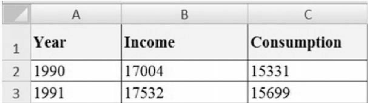
Figure 6.1. Income and consumption data.
Enter income in cells B1 and consumption in C1, then save your work. Make a note of the full name of data and their sources for future reference. The best practice is to keep the original download file as it is and save the modified data in a separate spreadsheet or just another worksheet. Label each worksheet accordingly for reference. Make sure income is in column “B” and consumption is in column “C.” This assures that following the steps results in the same output as provided below. To perform a regression, execute the following commands:
Data → Data Analysis → Regression → OK
Enter the appropriate values in the drop-down boxes as indicated below:
Input X Range B1:B22
Input Y Range C1:C22
Click on the button on the left side of the “Label” to let the software know that the first row is a text containing variable names and not data. Click OK. The following result is provided in a new worksheet.
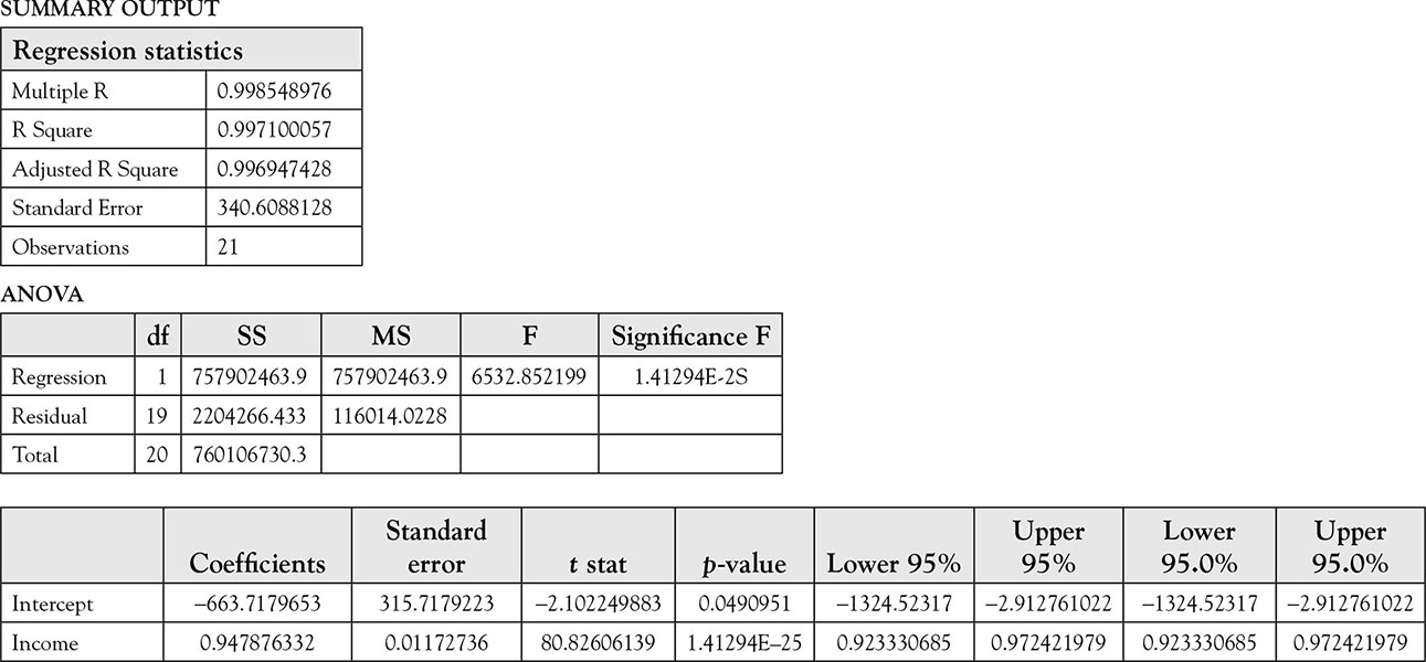
Analysis Regression Results for Estimating the Consumption Model’s Coefficients
The beginning point for regression analysis, as explained in Chapter 5, is the test for the following hypothesis:
H0: Model is not good H1: Model is good
The null hypothesis that the “model is not good” can be written as a set of complex hypotheses in terms of all the slopes of the model:
H0: μ1 = μ2 = … μk = 0 H1: At least one mean is different from zero
To test this hypothesis, examine the “significance F,” which is the Excel jargon for the probability of committing a type I error, if the above null hypothesis is rejected. The listed level of significance is 1.41294E–25, which means that the decimal place must be moved 25 places to the left of where it is shown. This is extremely low, and we reject the null hypothesis that the model is not good in favor of the alternative hypothesis, which states the model is good. This means that at least one of the independent variables has a coefficient that is not zero. However, the model only has one independent variable, which by default must have a slope that is not zero. Nevertheless, it helps to go through the steps of interpretation of the results. Following the same procedures will ensure proper analysis and reinforce the practice.
It is a good habit to write the estimated equation. It is usually what is reported in a published work. Customarily, the calculated t statistics are reported in parentheses under the equation. A better practice is to report the p values instead.
|
(6.5) |
The values in parentheses under the estimated equations are the p values for each estimated parameter. Some people prefer standard errors, others prefer t statistics, but this author prefers p values, which can be used directly and without the need for further computation or use of reference tables to make an inference. Some people would immediately proceed to explaining the meaning of the coefficients. This is a poor practice. The magnitudes of coefficients are really meaningless if one cannot reject the null hypothesis that they are equal to zero. The hypothesis about the slope is
H0: MPC = 0 H1: MPC > 0
Or equivalently in symbolic form:
H0: β1 = 0 H1: β1> 0
The p value associated with MPC is small, and we should feel confident in rejecting the null hypothesis. The probability of committing a type I error when rejecting this null hypothesis is a little over 1.4 in 1025, which is equal to a 1.4 with 25 zeros to the right of it; in comparison, the population of the world is 7 × 10⁹, which is 7 with only 9 zeros in front of it. Therefore, we should feel confident that rejecting the null hypothesis is the right thing to do. The conclusion is that MPC is not zero; it is positive. An observant student will notice that the probability of type I error for the t statistics for the slope of the independent variable, that is, income is the same as the p value for the F statistics. This is always true for the case of a single independent variable, as elaborated in Chapter 5.
After rejecting the null hypothesis that the slope is zero, it is possible to examine its meaning. The slope of 0.95 means that Americans will spend 95 cents of every additional dollar they earn and save the rest, which is 5 cents. A better way of looking at this aspect of the results is through a confidence interval. We chose not to change the default level of confidence, which happened to be 95% for Excel as default. The 95% confidence interval for the real MPC is between 0.92 and 0.97 in the above example; the range 92–97 cents includes the real MPC with 95% confidence. It is a coincidence that MPC is 95%, which is the chosen level of confidence.
Test of Hypothesis About Intercept
The procedure for testing a null hypothesis about intercept is exactly the same. If the probability of committing type I error is small, reject the null hypothesis; if not, fail to reject it. But what are the null and alternative hypotheses for intercept?
The simplistic consumption equations of (6.1) and (6.2), and therefore, their corresponding statistical model expressed in equation (6.4) indicate that if one’s income is zero, he or she would consume an amount equal to β0, which represents the subsistence level, at least in the macroeconomic theory of consumption. This implies that the subsistence level of income should be low and positive. In fact, the idea of a negative consumption is absurd. So a reasonable claim about the subsistence level is that it should be positive, or greater than zero. The number that nullifies this claim is zero. Therefore,
H0: β0 = 0 H1: β0 > 0
Once again, note that the process began with the alternative hypothesis. After establishing an appropriate alternative hypothesis based on some economic theory, the value that nullified it is stated as the null hypothesis. This test really does not require any computation. The claim is that the intercept is positive, but regression estimate in equation (6.5) is negative. Therefore, there is no evidence to support a positive intercept based on the data from the years 1990–2010. A negative number can never provide any support for a claim that the true level of subsistence is positive no matter how far it is from the center. Thus, we fail to reject the null hypothesis. If we reject the null hypothesis, the probability of type I error is a little over 50%. In fact, it is exactly:
0.5 + 0.04909 = 0.54909
Some Common Mistakes
The novice often refers to the output and observes a negative number in front of the estimated intercept and then chooses the following (incorrect) null and alternative hypotheses:
H0: β0 = 0 H1: β0 < 0
He/she proceeds by observing the reported p value of 0.04909, which is a small probability, and rejects the null hypothesis in favor of the alternative hypothesis. This is incorrect because there is no economic theory that explains a negative subsistence level.
The original claim is the correct claim, and the theory anticipates a non-negative consumption in spite of lack of income, which also makes common sense. However, there is not sufficient evidence to reject the null hypothesis that when one’s income is zero his or her consumption is zero as well. In other words, according to the estimated equation, when income is zero one ceases to consume and dies. This is a plausible, although it is an oversimplification of reality, at least in the short run. In the short run, one would not die as a result of lack of income. Even with zero consumption, it would take a while for death to occur. Where the model clashes with reality is in the fact that the model ignores the possibility of having savings, wealth, family, relatives, and not to mention theft. The appropriate thing to do would be to improve the model by including the above-mentioned control variables in the model, rather than jumping to an illogical conclusion.
Another common mistake is to look at the magnitude of –663.717 (the coefficient of the intercept from Table 6.1) and conclude that it is large. Because measurements are in dollars, this number reflects a negative $663.71. Although not a fortune by any stretch of imagination, it is nevertheless a far cry from a zero dollar consumption of the null hypothesis. The fact is that in order to have an average = 0, one must observe some negative values and some positive values in such a way that the average is zero. In this example, it happens that the observed estimate is negative. The magnitudes of positive and negative values depend on the variance of the data. The more problematic issue is the fact that the estimate has a relatively small standard error as compared to the coefficient, namely 315. This results in a relatively large t statistic of –2.10. Although, as explained above, this evidence cannot be used to conclude a positive subsistence consumption level, nevertheless, it would make one uncomfortable stating that the intercept is zero. This is further evidence that when we fail to reject the null hypothesis, we need to be cautious and not conclude that the null hypothesis is accepted.
Table 6.1. The Results of Regression of Per Capita Personal Consumption Expenditures on Per Capita Income 1990–2010
For this and other reasons to be explained later, there is little stock placed in interpretation of the intercept of a regression model in many instances. Instead, the main focus is on the slope, and whether it is zero. A zero slope indicates the failure of an independent variable to explain variation in dependent variable; indicating that inclusion of that particular variable does not improve the explanatory power of the model. Therefore, the best variable to explain variation in the dependent variable is its mean.
One should not form a claim, that is, an alternative hypothesis, based on empirical evidence from a sample. The claim must be made before the data are collected. Also, alternative and null hypotheses must be stated first. Otherwise, an error will be made by rejecting the null hypothesis using the incorrect alternative hypothesis, which is known in the literature as the type III error.
Definition 6.1
A type III error is rejecting a null hypothesis in favor of an alternative hypothesis with the wrong sign.
Coefficient of Determination: R2
Coefficient of determination shows what percentage of variation in dependent variable is explained by a regression model. In this case, 99.88% of variations in consumptions are due to differences in income. This is an impressive performance for a humble model. It is important to know that when two variables increase overtime, they will do a good job explaining variations in each other. This occurs in time series data frequently. Therefore, other things being equal, R2 would be higher for time series data, such as income and consumption from 1990 to 2010 in this example. The problem will be addressed in greater detail in Chapter 9, Spurious Regressions.
A low value of R2 indicates, among other things, that a small percentage of changes in the dependent variable are explained by a regression model. However, a high value of R2 can either mean a high explanatory capability or it could be due to other factors, one of which is addressed in the next paragraph. The terms “low” or “high” are indeterminate and vague. Because 0 ≤ R2 ≤ 1, the extreme values for low and high end are known. What is not known is how close the value of R2 must be to zero before it is considered low, and how close it should get to one to be considered high. Statements about the explanatory power of R2 are one of the rare occasions where no probability is provided for the accuracy of the statement. Therefore, they lack the precision of statements associated with F statistics, for which probabilities of type I and type II can be calculated and a power of a test determined.
Another problem with the use of R2 is that it gives a point estimate and does not have a familiar or commonly used confidence interval. However, there is a relation between R2 and F value as expressed in Chapter 5 under the section Relation between R2 and F.