
Regression Assumptions
Need for Assumptions
This appendix explains necessary assumptions about error term in regression analysis and addresses other important issues that are essential for correctness of the results. In order to be able to use theories in statistics to perform statistical analysis, it is necessary to adhere to the rules that govern those theories or are prerequisite for their validity. The assumptions that are listed and discussed below are necessary for validity of inferences. The proofs of their contribution to the theory and the validity of the conclusion are left for specialty textbooks. However, before addressing the assumptions, let us change the notation of equation (1.9)
C = β0+ β1Y + ε(A.1)
to a more generic equation where the dependent variable is designated by the letter Y, and the independent variable is designated by the letter X. In this formulation, the letters “Y” and “X” are merely placeholders for the dependent and independent variables, respectively.
Y = β0+ β1X + ε (A.2)
Assumption A.1
In a regression model, the relationship between dependent and independent variables is linear in parameters. The model in (A.2) is an example where the linearity assumption is met.
The linearity assumption is different from the definition of a line, which requires the powers of X and Y to be equal to one. The following model still meets linearity assumption and is considered a linear regression model, while it does not represent a line in geometric sense.
Y = β0+ β1 X 2 + ε.(A.3)
Functions with powers of 2 are known in mathematics as quadratic functions. To see how model (A.2) meets the linearity assumption, we define a new variable Z = X 2.
Y = β0+ β1Z + ε.(A.4)
Model (A.4) is identical to model (A.2).
Assumption A.2
Data are obtained by random sampling. This means that observation must be chosen at random. It does not mean that the observations must be random.
Assumption A.3
Conditional expected value of the error given the independent variable is zero. The key concept here is conditionality. It means that given a particular value of an independent variable, the average of the error term is zero. The conditional relationship between the error term and the independent variable is extended to a conditional relationship between the dependent variable and independent variable. In other words, for a given value of X there exist many potential values of Y, one of which is observed in the sampling pair (X, Y ).
The consequence of this assumption is that conditional expected value of the dependent variable given the independent variable is
E(Y |X) = β0+ β1X.(A.5)
The estimated “expected” value of Y from regression is
|
(A.6) |
Assumption A.4
The conditional variance of the error given the independent variable is constant σ2.
The consequence of this assumption is that conditional variance of the dependent variable given the independent variable is
Var(Y |X )= σ2 |
(A.7) |
Another common way of stating the above assumptions is to say that the dependent variable is a linear function of the independent variable where the random errors of the model have independent and identical distribution with mean zero and a constant variance, which is depicted by σ2.
Statements in assumptions A.3 and A.4 involve the word conditional. This is very important because without requiring the presence of an independent variable the only statement we can make about the dependent variable would be based on observations of the dependent variable. This reduces to statements based on the average of dependent variables.
For example, in the model about consumption
Consumption = β0+ β1 Income + ε |
(A.8) |
Assumptions A.3 and A.4 state that for every value of income there are many possible values of consumption. The actual observed value of consumption is just one of those possibilities chosen at random. The expected value of a particular consumption value is given by E (consumption) = β0 + β1 Income. If the endogenous variable (consumption) did not depend on the exogenous variable (income) the best estimate for the endogenous variable would have been its mean (average consumption). However, because the dependent variable is conditional on the exogenous variable, the best linear estimate is the regression line.
Parameters β0 and β1 are usually unknown and must be estimated by regression analysis, which, according to Chapter 3, are estimates with some desirable properties. One such desirable property is the fact that the mean of squared error is the smallest possible mean squared error when the method of least squares is used. More detail on this issue is discussed below.
Assumption A.5
It is essential that the error term be random. The error term is not the same as error. The definition of error is repeated below:
Error is the proportion of variation among the values of the dependent variable that cannot be explained.
In Chapter 2, several distinct but related “errors” or error-based concepts were discussed. All of these “errors” are statistics, which indicates that they are obtained from samples. Some of the “errors” have specific names based on their origin and use, such as variance or sum of squared residuals. Many errors have several names or could be called by other names, meaningfully, such as standard deviation, which is also the average error. The standard deviation represents the average error of using the mean to predict or estimate observations. All of these “errors” are actually random variables in their strict statistical terms; they are obtained from a sample and are known by virtue of computation of observed values.
The error term in a regression model, however, is a property of the model. The error term is not observable and does not come from a sample, although it can be estimated using sample data and regression analysis. The estimated values are statistics, which were mentioned in the previous paragraph
It is of vital importance not to mistake any of the concepts of errors with errors in measurement. Errors in measurement refer to incorrectly measured or recorded values of dependent or independent variables. In some social science disciplines, the measurement error is called validity. It is also important to note that the only requirement for randomness is for the error term. There is no assumption or requirement that independent variables be random. In fact, if independent variable were random it would introduce the possibility that it is not independent from the error term, which has some serious consequences. There is no randomness requirement for the dependent variable either. However, the dependent variable, by virtue of being a linear function of the error term and the randomness requirement of the error term, also becomes a random variable. The dependent variable has the same distribution function as the error term with the following properties:
E(Y |X ) = β0+ β1X (A.9)
Var(Y |X )= σ2 (A.10)
We still have not addressed the distribution function of the error term because none of the discussion so far required any particular distributional properties. Nevertheless, like any random variable, the error term has a distribution function that governs and determines the outcome and the value of what is observed. The distribution function could be, and in fact for most real-life events, is unknown. The discussion about the properties and consequences of distribution function of the error term is limited to the ones that are either known or can be approximated by a known distribution function.
The main need for assumptions about error term is to allow using mathematical statistics to derive desirable properties for the estimates of parameters of the model. If the estimates of parameters lack these desirable properties, they are useless for all practical purposes.
Desirable Properties of Estimators
A statistics, as defined above, provides an estimate for population parameter. A more correct term is a point estimate. There are three properties that make a point estimate useful. An estimate must be unbiased, consistent, and efficient. Estimators that can assure these properties are considered desirable estimators. These terms have precise definitions with assumptions and conditions that are the subject of mathematical statistics. Here, however, strict definitions and necessary assumptions are relaxed for the sake of simplicity. All estimates are variables because they are obtained from sample data; they are statistics. They are used to make inferences about their corresponding parameters, which are characteristics of population and are always constant.
Definition A.1
Unbiasedness
An estimate is an unbiased estimate of the corresponding population parameter if its expected value is equal to the population parameter.
For example, the sample mean is an unbiased estimate of population mean.
|
(A.11) |
The expected value of an unbiased slope of a regression equation (a statistics) is equal to the slope of regression model (a parameter).
|
(A.12) |
Theorem A.1
If error terms in a regression model are independent, then the estimated slopes and estimated intercept are unbiased estimates of slopes and intercept of the regression model.
|
(A.13) |
|
(A.14) |
Failing to comply with the assumption would make the theorem inapplicable.
Definition A.2
Consistency
An estimator is a consistent estimator if its variance becomes smaller as sample size increases.
For example, the sample mean is a consistent estimator of the population mean. Because variance is a measure of error, as sample size increases, the error of sample mean in estimating population mean becomes smaller.
Theorem A.2
If the error terms of regression model are independent, then the estimated slopes and the estimated intercept are consistent estimates of the slopes and the intercept of the regression model.
Therefore, the error of estimated slope becomes smaller as sample size increases. Eventually, as sample size approaches infinity, estimates of slopes approach slopes of the population.
Definition A.3
Efficiency
Efficiency is a comparative property. An estimate is said to be more efficient than another estimate if its variance is smaller than the variance of the other estimator. Sample mean is the most efficient estimator of population mean among all its unbiased estimates. This does not preclude the existence of a more efficient but biased estimate for population mean.
Theorem A.3
If error terms in a regression model are independent, then among all the unbiased estimators of the intercept and slopes of the model, the least square estimates are the most efficient estimates.
In other words, slopes and intercept estimates obtained by the method of least square have the smallest variances among all the unbiased linear estimators of the slopes and intercept. These estimates are called the best linear unbiased estimators (BLUEs). The text provided two examples for estimating consumption. One was the average consumption and the other was the regression estimates. The estimates obtained using regression based on the slope and intercept from the least square methods have smaller variances than the estimates based on the average consumption.
The theorems that are listed above are broader than the form in which they are presented here. An important point to remember is that no specific distribution function has been required for the error term. Often, econometric books submit the above into a single theorem called Gauss–Markov theorem. If the assumptions are not valid or if the rules are broken, then the premises of the Gauss–Markov theorem would not hold either.
Violations of Regression Assumptions
The presumption in this book is that the assumptions for regression analysis are met. In this section, a brief discussion of consequences of violating some of the regression assumptions is presented. Detecting and remedying the problems caused by such violations are beyond the scope of this book, as they require more sophisticated and specialized software than Excel.
Assumption A.6
The distribution function of the error term is normal with mean μ and variance σ2. By far, the assumption of normality is the most important assumption because without it the goodness of fit of regression cannot be tested using the F statistics. It is also impossible to test hypotheses about regression coefficients using t statistics; the same is true about building confidence intervals for the model or for the parameters.
The consequence of normality assumption for error term is that the dependent variable, Y, has a normal distribution as well. The variance of the dependent variable (Y) values is the same as the error term, namely σ2. However, the expected value of the dependent variable is
E(Y) = β0+ β1X |
(A.15) |
Therefore, there are as many expected values for Y as there are pairs of data. For each value of independent variable (X) there are infinite possible values of Y, all of which come from the governing normal distribution having an average equal to β0+ β1X and a variance equal to σ2. Figure A.1 below depicts the relationship. The line that connects the expected values of the Y’s, that is, the conditional means of each Y distribution corresponding to each of the X values, is the regression line.
Figure A.1. Conditional distribution of Y with normality assumption.
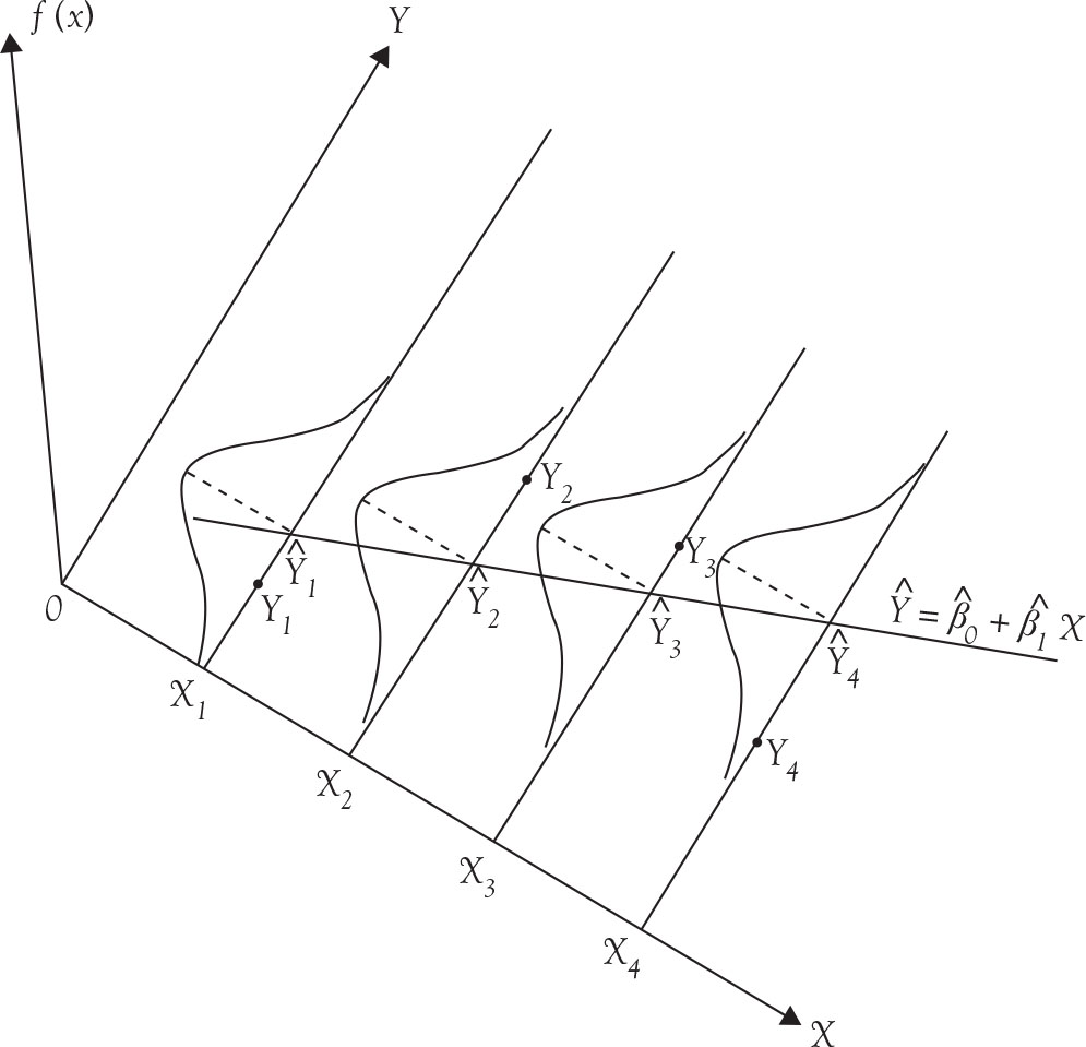
Note in Figure A.1 that the spread or the variances of the Y values depicted by the four normal distribution functions are the same.
Testing and Remedy for Violations of Normality
One of the ways to check for violations of normality is through tests for skewness and kurtosis.1 Both statistics can be calculated in Excel using Skew and Kurt functions. The skewness and kurtosis tests refer to deviation from symmetry and pointedness, as compared to normal distribution, respectively. Kolmogorov–Smirnov and Shapiro–Wilk tests are two nonparametric tests of normality. These statistics, although simple to calculate, are not available in Excel, but online help with instructions to perform these tests are available. Another alternative is to consult one of the dedicated statistical analysis software.
Some textbooks suggest graphical inspections using numerous available graphs. This practice is a waste of time. The experts need to be able to test the hypothesis of normality precisely; a novice lacks the experience to differentiate between a normal and non-normal distribution by viewing graphs, except when the violation is flagrant. In cases of possible violation of this and other regression analysis assumptions, the reader is advised to move to the next level and gain the necessary knowledge to test the possibility of violation and to solve the problem.
Under some conditions, and in simple cases, transforming data in a monotonic way such as taking natural logarithm might improve the situation. If normality cannot be established, tests of hypotheses are meaningless and nonparametric methods must be incorporated.
Heteroscedasticity or Violation of Constant Error Variance
The assumption that variances of error term are constant, which is also known as homoscedasticity, is an important one. The problem of heteroscedasticity, or lack of equal variances, is more prevalent in cross-section data than in time series data. The consequence of heteroscedasticity is that regression coefficients are inefficient, although they are still unbiased and consistent. As indicated earlier in this appendix, efficiency refers to the size of the variance of estimates of a parameter, in this case the slopes, compared to variances of other estimation methods. When error variance is large, slope variance is also large, which in turn makes t statistics small. Consequently, the statistics might not be large enough to be statistically significant and results in failing to reject the null hypothesis, erroneously—a type II error.
When heteroscedasticity is present, it can be shown that variances of slopes of regression are biased, invalidating the tests of hypotheses about parameters and confidence intervals.
Because variances are different in the presence of heteroscedasticity, the spread of the values for dependent variable are not the same. Compare Figure A.2 with Figure A.1 and notice the difference between the spreads of the normal distribution functions.
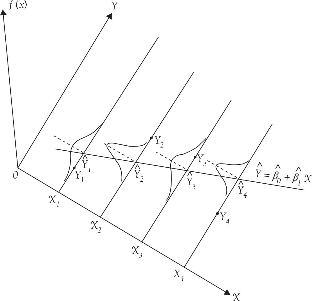
Figure A.2. Conditional distribution of Y under heteroscedasticity.
Testing and Remedy for Heteroscedasticity
The most common tests for heteroscedasticity are Breusch–Pagan test and White test. Neither is available in Excel and they require dedicated statistical software. The best solution to deal with heteroscedasticity is to use White’s robust procedure. This method is beyond the scope of this book.
Serial Correlation
Serial correlation is the violation of independence of error terms. Serial correlation is more common in time series data than in cross-section data, especially for adjacent time periods or in the case of cyclical data when the data points represent similar cycles, for example, the fourth quarter. In majority of time series data, the problem of positive or direct correlation is more common than the negative or inverse correlation. One possible source of serial correlation is the inclusion of a lagged dependent variable as an exogenous variable.
Serial correlation does not affect unbiasedness or consistency of regression coefficients. However, efficiency is affected. Variances of slopes are be biased downward, indicating that they are be smaller than the true variances, especially when there is positive serial correlation. Therefore, t statistics will be larger than usual and the null hypothesis of zero slope would be rejected more often than they should be, resulting in type I errors. Serial correlation does not affect the coefficient of determination or R2.
The serial correlation in time series is also called autocorrelation. Interestingly, the presence of autocorrelation can be used to provide better prediction for future values. In fact, some of the foundations of time series analysis are based on the use of serial correlation.
Testing and Remedy for Serial Correlation
There are numerous tests for different types of serial correlation, from a simple t test in the case of autoregressive of order one to a classical test of Durbin–Watson to Breusch–Godfrey test for higher order autoregressive cases. An autoregressive model is a time series model where the value of the endogenous variable is a weighted average of its own previous values.
The remedies also differ based on the situation. Some possible solutions when serial correlation exists include first differencing, generalized least squares, and feasible generalized least square (FGLS).