Instrumental Variable Method for Addressing Selection Bias
6.2 Overview of Instrumental Variable Method to Control for Selection Bias
6.4 Traditional Ordinary Least Squares Regression Method Applied to Case Study
6.5 Instrumental Variable Method Applied to Case Study
6.6 Using PROC QLIM to Conduct IV Analysis
6.7 Comparison to Traditional Regression Adjustment Method
Observational data can provide powerful answers to research questions when properly addressing selection bias due to non-randomization. The medical literature has relied mostly on conventional regression and propensity score methods, which rely on observed variables, to adjust for selection bias. Such methods might deliver biased estimates due to unmeasured confounding. In this chapter, we introduce the instrumental variable method, an econometric method, to adjust for selection bias and illustrate its use in evaluating treatment effects on medication compliance. If properly applied, this method might be more useful in addressing selection bias.
A key strength of observational studies is their ability to estimate the effect of treatments and interventions in real-world conditions. However, the lack of random group assignment may impose a serious threat to the results of observational studies (D’Agostino and Kwan, 1995). Non-randomized groups usually differ on observed and unobserved characteristics, which in turn result in differential selection into treatment groups. This non-random sampling selection is one form of selection bias that distorts the effect of treatment on outcomes. In other words, it is unclear whether the observed treatment effect is due to the treatment itself or to the differential selection into treatment groups due to non-randomization.
This selection bias problem has been shown to have a substantial impact on the treatment effect in some studies, while in other studies adjusting for selection bias has resulted in minor changes in the treatment effect (Wang, 2005; Foster, 2000; McClellan, 2000; Grimes, 2002; Glesby, 1996). Therefore, several studies caution that overestimating the selection bias may lead to further biased estimates (Hernán, 2006; Stukel, 2007). In this chapter, we provide an overview of instrumental variable (IV) methodology and demonstrate an example of applying this approach to adjust for selection bias using administrative claims data. The IV approach is an econometric method that is less prevalent in the medical literature than methods of matching, stratification, conventional regression, and propensity scoring, but it may have advantages over these methods if used appropriately.
6.2 Overview of Instrumental Variable Method to Control for Selection Bias
Observational studies that lack randomization of subjects into treatment groups must address selection bias to properly estimate the effect of treatment while addressing potential confounds. Instrumental variable (IV) analysis is a common tool in economics and social sciences to adjust for selection bias but less used in health care research. Where conventional selection adjustment methods use only observed variables, the IV method, on the other hand, acknowledges that a set of observed variables may not capture residual confounding due to unobserved factors (Angrist et al., 1996). By implementing the IV method, researchers find variables, called instruments or instrumental variables, which are highly correlated with the treatment selection but not directly correlated with the outcome variable. When incorporated into the analysis, the IV creates additional variance that is unaccounted for from the observables to obtain an unbiased estimate of the effect of treatment on the outcome. In 2000, the Health Services Research journal published a special supplemental issue devoted to IV analysis (McClellan and Newhouse, 2000). This issue contains explanations of the methodology and provides examples of its use in health outcomes research.
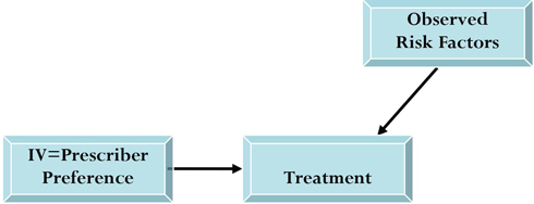
Figure 6.1 illustrates how an instrumental variable works. Observable risk factors or confounders (X) (such as age, gender, and co-morbid conditions) may affect both the outcome (Y) and treatment (T). The presence of this association makes treatment allocation dependent on observables and not truly an independent variable. That is, treatment is correlated with the error term in the model. Thus, estimating the effect of treatment (T) on outcome (Y) without any adjustment creates difficulty in deciphering cause and effect between treatment and outcome. Traditional regression methods can account for observables but won’t capture bias from unobservables. The goal of IV analyses is to find an instrument or instruments that are correlated with treatment selection but are not directly correlated with the outcome variable. These IVs are then used in estimating a treatment effect that is independent from the observables (X). The objective is to mimic randomization of subjects into treatment groups to be able to attribute changes in outcome due to treatment rather than observables.
Figure 6.1 Schematic Representation of IV Methodology

While the intuition of IV methodology is appealing, the difficulty in finding a valid instrument may be the reason for its relatively limited use. For the IV method to overcome unmeasured confounding, several assumptions must be addressed (Angrist, 1996; Landrum, 2001; Greenland, 2000). Most noteworthy assumptions include the independence assumption, exclusion restriction, and non-zero causal effect of the instrument on treatment. The independence assumption states the lack of relation between the instrument and the observed risk factors. The exclusion restriction requires that the IV have no effect on the outcome other than through treatment or that the IV affect the outcome exclusively through treatment. The non-zero causal effect of the instrument on treatment assumes that the instrument is associated with treatment or a predictor of treatment.
In order to estimate a treatment effect that is adjusted for selection bias using the instrumental variable approach, two equations need to be estimated. The first equation estimates the effect of the IV and observables (X) on treatment (T). The second equation estimates the effect of observables (X) and treatment (T) on outcome (Y). The maximum likelihood ratio method is usually used in conducting this two-stage regression estimation of treatment on outcome. Using the Heckman two-stage estimation to calculate the inverse Mills ratio is another way to accomplish the IV approach (Heckman, 1978).
The remaining sections of this chapter discuss an example of using the instrumental variable methodology to evaluate the effect of drug choice on medication adherence in a population of diabetic patients. Determining differences between treatments is important because increased adherence to medications may indicate better diabetes disease management, which consequently may slow disease progression. These data are often used when deciding on a preferred treatment for larger populations. We conducted our instrumental variable analysis using the Qualitative and Limited Dependent Model (QLIM) procedure in SAS/ETS.
A large pharmacy claims database was used to identify newly started patients using one of two oral antidiabetic medications in a 7-month time period (N=19,433). The purpose of the study was to compare compliance rates over a 180-day period between the two treatments. Compliance was measured as the proportion of days a medication was covered or supplied to the patient after treatment initiation (Benner, 2002). Patients new to therapy, or new starts, were chosen for review because this sample gives a more accurate estimate of initial compliance with the medication. New starts are also less confounded by previous medication use and more exposed to selection of treatment through the prescriber. We suspected the presence of selection bias because evidence shows the two drug treatments differ in patient tolerance, adverse events, and side effects, which possibly influence treatment selection as well as compliance with each drug (Lago et al., 2007; Lincoff et al., 2007). Additionally, selection of treatment is influenced by recent findings, changes in clinical guidelines, and policy changes (Schneeweiss, 2002). Knowing that traditional regression techniques may fall short in estimating the treatment net effect on the outcome, we chose the IV approach to minimize bias attributed to unmeasured data.
The TABULATE procedure code in Program 6.1 was used to create a table displaying patient characteristics by drug treatment for the new starts sample. Additionally, PROC TTEST and PROC FREQ were used to test for differences and associations between groups. Descriptors include demographic variables (age, gender), type of health plan insurance, and medication use in a 6-month period prior to treatment initiation (baseline period). Age was the age of the patient at date of treatment initiation (index date). Type of insurance was categorized by health maintenance organization (HMO) or other. Prior medication use was measured for sulfonylureas, antihypertensives, lipid lowering agents as well as asthma and antidepressant medications. Refill patterns of medications for chronic diseases, or maintenance medications, were used to estimate patient compliance behavior with the following prescribed dosings.
Program 6.1 Displaying Patient Characteristics by Drug Treatment Using PROC TABULATE
proc format;
picture pct 0-100=009.0% (mult=1000);
run;
proc tabulate data=newstarts;
class tx;
var age age_18to44 age_45to54 age_55to64 age_65plus b_hmo b_medicaid
b_medicare b_self pre_sulf _0106 _0109 _0112 _0113 _0149 female
maintrefillratio pre_stc_class_cnt_subset pre_drug_cnt_subset;
table N='Member Count'*f=comma8.
(age='Age')*(mean std='SD')*f=4.1
(age_18to44='Age Group 18-44' age_45to54='Age Group 45-54'
age_55to64='Age Group 55-64' age_65plus='Age Group >=65'
female='Female')*(mean='')*f=pct.
(b_hmo='HMO Enrollee')*(mean='')*f=pct.
(pre_drug_cnt_subset='# of Drugs Utilized')*(mean std='SD')*f=4.1
(maintrefillratio='Maintenance Medication Refill %')*(mean='')*f=pct.
(pre_sulf='Sulfonylurea' _0106='Hypertension' _0109='Lipid
Irregularity' _0112='Pain Management' _0113='Antidepressant'
_0149='Asthma')*(mean='')*f=pct.
, tx='Treatment' /box='Unadjusted Demographic and Baseline
Characteristics';
run;
proc ttest data=newstarts;
var age pre_drug_cnt_subset maintrefillratio;
class tx;
proc freq data=newstarts;
tables tx*(female b_hmo pre_sulf _0106 _0109 _0112 _0113 _0149)/chisq;
run;
Output from Program 6.1
| Unadjusted Demographic and Baseline Characteristics | Treatment | ||
| Drug A | Drug B | ||
| Member Count | 611 | 815 | |
| Age | Mean | 55.5 | 56.0 |
| SD | 11.8 | 12.6 | |
| Age Group 18-44 | 16.3% | 16.3% | |
| Age Group 45-54 | 30.9% | 28.3% | |
| Age Group 55-64 | 32.8% | 34.1% | |
| Age Group >=65 | 19.8% | 21.2% | |
| Female | 44.6% | 46.3% | |
| HMO Enrollee * | 65.3% | 74.8% | |
| # of Drugs Utilized | Mean | 3.1 | 3.3 |
| SD | 3.1 | 3.8 | |
| Maintenance Medication Refill % * | 36.3% | 41.3% | |
| Sulfonylurea | 27.6% | 31.5% | |
| Hypertension | 56.6% | 57.7% | |
| Lipid Irregularity | 34.5% | 38.7% | |
| Pain Management * | 21.1% | 26.1% | |
| Antidepressant | 14.5% | 13.6% | |
| Asthma * | 7.2% | 10.6% | |
* p < .05
Output from Program 6.1 describes the two treatment groups. Those observables that differed significantly in the two groups of patients include type of insurance (proportion of patients enrolled in an HMO), previous refill rate for maintenance medication, asthma medication use, and pain medication use. Differences in observables between groups led us to believe differences existed in unobservables between the two groups.
To compare methods to control for selection bias, our analytic plan proceeds as follows. We use three methods in estimating the difference in outcome between Drug A and Drug B. First, a simple t-test crudely compares the mean compliance rates for drugs A and B using PROC TTEST. Second, we use conventional ordinary least squares regression to compare drug effectiveness on compliance for Drugs A and B, adjusting for measured covariates. Third, we estimate compliance rates for the two treatments, adjusting for selection bias using the IV method.
Our compliance outcome was measured as the proportion of days the medication was supplied over the 180-day period; hence, the maximum allowable value was 1. Mean compliance for Drug A and Drug B was 0.4774 and 0.5122, respectively. The unadjusted comparison of mean compliance values using PROC TTEST (Program 6.2) indicates the difference is approaching statistical significance (p = 0.0609) at the 0.05 level of significance. This unadjusted 3% difference in compliance between treatments indicates better compliance to prescribed dosings, which may translate into better diabetes disease management. Such evidence can influence formulary management decisions on the preferred treatment for large populations. Displaying distributions of the outcome for the two treatment groups can be done using the CLASS statement in PROC UNIVARIATE, as shown in Program 6.2.
Program 6.2 Computation of t-test Comparison of Mean Compliance Values and Generation of Histograms
proc ttest data=newstarts;
var pdc;
class tx;
proc univariate data=newstarts noprint plot;
var pdc;
class tx;
histogram pdc / ctext=purple cfill=blue
kernel (k=normal color=green w=3 l=1)
normal (color = red w=3 l= 2)
ncols=1 nrows=2;
inset n='N' (comma6.0) mean='Mean' (6.2) median='Median' (6.2)
mode='Mode'(6.2)
normal kernel(type)/ position=NW;
run;
Output from Program 6.2
The TTEST Procedure
Statistics
| Variable | tx | N | Lower CL Mean |
Mean | Upper CL Mean |
Lower CL Std Dev |
Std Dev | Upper CL Std Dev |
Std Err |
| pdc | Drug A | 611 | 0.4494 | 0.4774 | 0.5055 | 0.3345 | 0.3532 | 0.3742 | 0.0143 |
| pdc | Drug B | 815 | 0.4887 | 0.5122 | 0.5356 | 0.3248 | 0.3405 | 0.3579 | 0.0119 |
| pdc | Diff (1-2) | -0.071 | -0.035 | 0.0016 | 0.3338 | 0.346 | 0.3592 | 0.0185 |
T-Tests
| Variable | Method | Variances | DF | t Value | Pr > |t |
| pdc | Pooled | Equal | 1424 | -1.88 | 0.0609 |
| pdc | Satterthwaite | Unequal | 1288 | -1.87 | 0.0623 |
Equality of Variances
| Variable | Method | Num DF | Den DF | F Value | Pr > F |
| pdc | Folded F | 610 | 814 | 1.0 8 | 0.3317 |

6.4 Traditional Ordinary Least Squares Regression Method Applied to Case Study
Using ordinary least squares regression methods to adjust for observed risk factors, we obtained adjusted estimates of compliance for the two treatment groups. The GLM procedure can conduct an analysis of variance to calculate least squares means while using the Tukey-Kramer (Kramer, 1956) adjustment for multiple comparisons (Program 6.3). Tests of univariate associations with the outcome were used to select the independent variables in this model.
Program 6.3 Creating Adjusted Outcome Values Using PROC GLM
proc glm data=newstarts;
class tx age_18to44 female b_hmo pre_sulf _0112;
model pdc = tx age_18to44 female b_hmo maintrefillratio _0112
/solution;
lsmeans tx/OM ADJUST=TUKEY PDIFF CL;
quit;
Output from Program 6.3
The GLM Procedure
Least Squares Means
Adjustment for Multiple Comparisons: Tukey-Kramer
| tx | pdc LSMEAN | H0:LSMean1= LSMean2 Pr > |t| |
| Drug A | 0.47863394 | 0.0747 |
| Drug B | 0.51124635 |
| tx | pdc LSMEAN | 95% Confidence | Limits |
| Drug A | 0.478634 | 0.451623 | 0.505645 |
| Drug B | 0.511246 | 0.487889 | 0.534604 |
Least Squares Means for Effect tx
| i | j | Difference Between Means |
Simultaneous 95% Confidence Limits for LSMean(i)-LSMean(j) |
|
| 1 | 2 | -0.032612 | -0.068480 | 0.003255 |
Adjusted compliance means for Drug A and Drug B are 0.4786 and 0.5112, respectively. The difference between means using the Tukey-Kramer adjustment shows no statistically significant difference in mean compliance values. Comparing these adjusted mean values to unadjusted mean values (Section 6.3) shows little change when adjusting for these observables.
6.5 Instrumental Variable Method Applied to Case Study
Suspecting that selection bias is not resolved with standard ordinary least squares methods, we employed the IV method. Among the few studies that apply the IV approach when comparing the treatment effectiveness of drugs, Brookhart and colleagues (2006, 2007) used physician prescribing preference as an instrumental variable when assessing drug treatment effectiveness on morbidity and mortality outcomes. The authors used these preference-based instruments in two separate studies to assess the risk of gastrointestinal toxicity associated with nonsteroidal anti-inflammatory drug treatment and the mortality in elderly patients using types of antipsychotic medications. Replicating their instruments, we used the last prescription written by the prescriber for the drug class (Drug A or Drug B) as the instrument for our study. Brookhart and colleagues hypothesized that a physician’s immediate history of prescribing as measured by the last written prescription estimates the prescriber’s preference for one treatment or another. That choice, according to the hypothesis, therefore, affects the choice of treatment for the prescriber’s next patient. We believed that in our study this measure would act as a valid instrument because it influences the treatment choice but is uncorrelated with the outcome for the next patient. To construct our IV, prescribers of the initial prescription for each of the 1,426 study patients were identified. Prescription claims for these prescribers for the two drugs were extracted in a period preceding this initial prescription to calculate the prescriber’s preference. Prescribers were classified as a Drug A prescriber or a Drug B prescriber based on their most recent prescription in the drug class. Some prescribers were not identified correctly. Some prescribers had no history of prescribing either drug; therefore, patients with these physicians were excluded from the analysis. A total of 1,226 prescribers were classified.
As stated earlier, the validity of an instrumental variable relies on many assumptions. Administrative data can’t confirm these assumptions, but they can be used to look into the credibility of the assumptions. To test the validity of our method, we first looked at the distribution of the IV to show that prescribers’ preference to prescribe these two drugs varied. Preference for Drug A or Drug B for the 1,226 identified prescribers was 47% and 53%, respectively. To address the non-zero causal effect of IV treatment assumption, we evaluated associations between the instrument and treatment selection by using PROC FREQ to estimate how well our instrument predicted treatment or the extent of prescriber preference in predicting the treatment choice of the prescriber’s next patient (Program 6.4). Results showed a strong, positive relationship between our IV and treatment selection. Prescribers with a preference for Drug A were more than three times more likely to prescribe Drug A for the identified patient in our sample (OR = 3.44, CI = 2.766 – 4.293).
To address the independence assumption, we checked relationships between our IV and observables factors. Potential violations of the independent assumption could include differing patient profiles by prescriber group (that is, Drug A prescribers treating patients who are much different than patients seen by Drug B prescribers). A stratification of patient demographic and baseline characteristics by prescriber preference using the TABULATE, TTEST, and FREQ procedures can compare observables by the instrument. More complicated models can address time variant clustering relationships (Brookhart, 2007). Smaller differences between groups indicate treatment choice by the prescriber for the previous patient is unrelated to the observables of the current patient. Those differences that persist suggest possible violations of this assumption; however, those covariates can be addressed later in the two-stage least squares regression.
The exclusion restriction requires that our IV have no effect on the outcome other than through treatment. Prescriber preference may be correlated with physician skill or other preferences of the prescriber that may affect outcome (Brookhart, 2006). Prescriber preference might affect compliance through other services provided by the prescriber or because of differing skill level among providers. However, review of the literature shows patients’ long-term adherence to medications is mostly due to the self-efficacy of the patient or the patient’s beliefs and behavior (Bodenheimer et al., 2002; Jerant et al., 2005) rather than instruction by the prescriber (Haynes, 2002). The degree of physician skill on our compliance outcome is difficult to measure so we use this research to defend the possibility of violating the exclusion restriction.
Program 6.4 Code Used in Validating IV Assumptions
proc freq data=newstarts;
tables iv*tx/chisq measures;
run;
proc format;
picture pct 0-100=009.0% (mult=1000);
run;
proc tabulate data=newstarts;
class tx iv;
var age age_18to44 age_45to54 age_55to64 age_65plus b_hmo b_medicaid
b_medicare b_self pre_sulf _0106 _0109 _0112 _0113 _0149 female
maintrefillratio pre_stc_class_cnt_subset pre_drug_cnt_subset;
table N='Member Count'*f=comma8.
(age='Age')*(mean std='SD')*f=4.1
(age_18to44='Age Group 18-44' age_45to54='Age Group 45-54'
age_55to64='Age Group 55-64' age_65plus='Age Group >=65'
female='Female')*(mean='')*f=pct.
(b_hmo='HMO Enrollee')*(mean='')*f=pct.
(pre_drug_cnt_subset='# of Drugs Utilized')*(mean std='SD')*f=4.1
(maintrefillratio='Maintenance Medication Refill
%')*(mean='')*f=pct.
(pre_sulf='Sulfonylurea' _0106='Hypertension' _0109='Lipid
Irregularity' _0112='Pain Management' _0113='Antidepressant'
_0149='Asthma')*(mean='')*f=pct.
, iv='IV (Prescriber Preference)' /box='Unadjusted Demographic and
Baseline Characteristics';
run;
Output from Program 6.4
| Table of iv by tx | |||
| iv | tx | Total | |
| Frequency Percent Row Pct Col Pct |
Drug A | Drug B | |
| Drug A | 390 27.35 58.56 63.83 |
276 19.35 41.44 33.87 |
666 46.70 |
| Drug B | 221 15.50 29.08 36.17 |
539 37.80 70.92 66.13 |
760 53.30 |
| Total | 611 42.85 |
815 57.15 |
1426 100.00 |
| Statistic | DF | Value | Prob |
| Chi-Square | 1 | 125.9656 | <.0001 |
| Likelihood Ratio Chi-Square | 1 | 127.5668 | <.0001 |
| Continuity Adj. Chi-Square | 1 | 124.7647 | <.0001 |
| Mantel-Haenszel Chi-Square | 1 | 125.8773 | <.0001 |
| Phi Coefficient | 0.2972 | ||
| Contingency Coefficient | 0.2849 | ||
| Cramer's V | 0.2972 |
| Estimates of the Relative Risk (Row1/Row2) | |||
| Type of Study | Value | 95% Confidence Limits | |
| Case-Control (Odds Ratio) | 3.4463 | 2.7665 | 4.2931 |
| Cohort (Col1 Risk) | 2.0138 | 1.7717 | 2.2890 |
| Cohort (Col2 Risk) | 0.5843 | 0.5281 | 0.6465 |
| Unadjusted Demographic and Baseline Characteristics | IV (Prescriber Preference) | ||
| Drug A | Drug B | ||
| Member Count | 666 | 760 | |
| Age* | Mean | 54.7 | 56.7 |
| SD | 11.7 | 12.6 | |
| Age Group 18-44 | 18.3% | 14.6% | |
| Age Group 45-54 | 28.5% | 30.2% | |
| Age Group 55-64 | 35.8% | 31.5% | |
| Age Group >=65 | 17.2% | 23.5% | |
| Female | 45.1% | 46.0% | |
| HMO Enrollee* | 66.0% | 74.8% | |
| # of Drugs Utilized | Mean | 2.8 | 3.5 |
| SD | 3.0 | 3.9 | |
| Maintenance Medication Refill % | 35.1% | 42.8% | |
| Sulfonylurea* | 26.7% | 32.6% | |
| Hypertension* | 53.0% | 61.0% | |
| Lipid Irregularity* | 33.0% | 40.3% | |
| Pain Management | 22.0% | 25.6% | |
| Antidepressant | 13.5% | 14.4% | |
| Asthma | 8.5% | 9.7% | |
* p < .05.
This output reinforces our choice of instrument for estimating treatment effectiveness in the presence of unmeasured confounding. Next, we applied the two-stage IV method to our study example. First, we used our instrument variable and other observables to predict the treatment (see Figure 6.2).
Figure 6.2 Schematic Representation of First Stage of IV Analysis
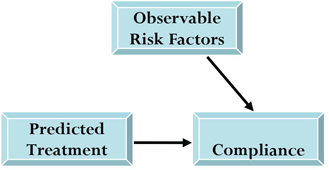
In the second stage of the process, an outcome equation approximates the compliance outcome by using the predicted treatment (from the first model) and other observables (see Figure 6.3). This two-stage approach has the advantage of incorporating the predicted treatment into the outcome model because it represents the portion of treatment selection related to prescriber preference.
Figure 6.3 Schematic Representation of Second Stage of IV Analysis
6.6 Using PROC QLIM to Conduct IV Analysis
The two-stage IV process described here can be done in one step using the Qualitative and Limited Dependent Model (QLIM) procedure in SAS/ETS. We chose the QLIM procedure because of its capability to analyze models that involve simultaneous relationships. This fits our example because we are simultaneously estimating treatment selection and compliance. The QLIM procedure let us submit two model statements in one procedure, allowing us to simultaneously estimate an unbiased effect of treatment on the outcome.
Proper modeling in PROC QLIM requires a subject-level data set (for example, one observation per patient). A quick look at the data set using PROC PRINT shows noteworthy variables of the data set (Program 6.5).
Program 6.5 Creating IV-Adjusted Outcome Value Using PROC QLIM
proc print data=newstarts (obs=10);
var tx druga iv pdc age female b_hmo copay_idxdrug
pre_drug_cnt_subset
pre_sulf _0106 _0109 _0112 _0113 _0149 maintrefillratio;
run;
proc qlim data = newstarts ;
class iv;
model druga = iv age female copay_idxdrug pre_drug_cnt_subset
maintrefillratio pre_sulf _0106 _0109 _0112 _0113 _0149 /discrete;
model pdc = age female copay_idxdrug pre_drug_cnt_subset
maintrefillratio pre_sulf _0106 _0109 _0112 _0113 _0149
/select(druga=0);
output out=drugb predicted;
run;
where
druga = treatment selection indicator
tx = treatment classification variable
iv = instrumental variable (prescriber preference)
pdc = outcome (compliance as proportion of days of medication covered)
age = age of patient at date of treatment initiation (index date)
female = indicator variable
b_hmo = HMO enrollee
copay_idxdrug = patient co-payment for initial prescription
Remaining variables describe utilization in the pre-treatment baseline period:
pre_drug_cnt = number of distinct medications utilized
pre_sulf = use of sulfonylurea
_0106 = use of antihypertensive
_0109 = use of asthma medication
_0112 = use of pain medication
_0113 = use of lipotropic
_0149 = use of antidepressant
maintrefillratio = refill percentage for maintenance medications
The first MODEL statement is a selection equation that uses the probit model (indicated by using the DISCRETE option) and creates the predicted probability of each subject receiving Drug B based on our IV and other observables. The second MODEL statement is the outcome equation, which uses linear regression to model the compliance outcome while controlling for covariates. This assesses the effect of the treatment while controlling for the probability produced from the first equation plus other believed confounders. Some believe that including independent variables other than the treatment group in this step is redundant because they are included in the first MODEL statement. We believe that adding variables to the model provides additional information on predictors of the outcome. The selection model can include covariates believed to be predictive of treatment where the outcome model can include covariates prognostic of outcome. The OUTPUT statement creates a data set named DrugB. With the addition of the PREDICTED option, the newly created data set includes all variables from the input data set plus two new variables named P_druga and P_pdc, which contain predicted values of the treatment and compliance values, respectively. The predicted compliance outcome values are generated for all subjects in the sample, assuming that all patients have been prescribed Drug B.
Output from Program 6.5
| Obs | tx | druga | iv | pdc | age | female | b_hmo | copay_idxdrug | pre_drug_cnt_ subset |
pre_sulf | _0106 | _0109 | _0112 | _0113 | _0149 | Maintrefill ratio |
| 1 | Drug A | 1 | Drug B | 0.00556 | 55 | 0 | 0 | 23.000 | 11 | 1 | 1 | 1 | 0 | 1 | 0 | 0.45946 |
| 2 | Drug B | 0 | Drug B | 0.16667 | 76 | 1 | 0 | 20.000 | 0 | 0 | 0 | 0 | 0 | 0 | 0 | 0.00000 |
| 3 | Drug A | 1 | Drug A | 0.07222 | 44 | 1 | 0 | 0.000 | 10 | 1 | 0 | 0 | 1 | 0 | 0 | 0.00000 |
| 4 | Drug B | 0 | Drug B | 0.91111 | 74 | 1 | 0 | 15.333 | 4 | 1 | 1 | 0 | 0 | 0 | 0 | 0.50000 |
| 5 | Drug B | 0 | Drug B | 0.16667 | 77 | 0 | 0 | 7.000 | 1 | 1 | 1 | 0 | 0 | 0 | 0 | 1.00000 |
| 6 | Drug A | 1 | Drug A | 0.61667 | 74 | 0 | 0 | 109.362 | 5 | 1 | 0 | 0 | 0 | 0 | 0 | 0.00000 |
| 7 | Drug B | 0 | Drug A | 0.16667 | 59 | 1 | 0 | 0.000 | 5 | 1 | 1 | 1 | 1 | 0 | 0 | 0.00000 |
| 8 | Drug A | 1 | Drug B | 0.28333 | 51 | 1 | 0 | 0.000 | 4 | 0 | 1 | 1 | 1 | 0 | 1 | 0.22222 |
| 9 | Drug B | 0 | Drug A | 0.27778 | 43 | 1 | 0 | 0.000 | 17 | 1 | 1 | 1 | 1 | 1 | 1 | 0.29167 |
| 10 | Drug A | 1 | Drug A | 0.16667 | 69 | 0 | 0 | 0.000 | 2 | 0 | 0 | 0 | 0 | 0 | 0 | 1.00000 |
| Parameter Estimates | |||||
| Parameter | Estimate | Standard Error | t Value | Approx Pr > |t| |
|
| pdc.Intercept | 0.468902 | 0.064961 | 7.22 | <.0001 | |
| pdc.age | 0.001444 | 0.000929 | 1.55 | 0.1201 | |
| pdc.female | -0.068086 | 0.022960 | -2.97 | 0.0030 | |
| pdc.copay_idxdrug | -0.001525 | 0.000305 | -4.99 | <.0001 | |
| pdc.pre_drug_cnt_subset | -0.001683 | 0.004240 | -0.40 | 0.6915 | |
| pdc.maintrefillratio | 0.168015 | 0.036034 | 4.66 | <.0001 | |
| pdc.pre_sulf | -0.042180 | 0.025716 | -1.64 | 0.1010 | |
| pdc._0106 | -0.001649 | 0.025733 | -0.06 | 0.9489 | |
| pdc._0109 | 0.047814 | 0.025504 | 1.87 | 0.0608 | |
| pdc._0112 | -0.045605 | 0.028238 | -1.61 | 0.1063 | |
| pdc._0113 | -0.008500 | 0.034562 | -0.25 | 0.8057 | |
| pdc._0149 | -0.006435 | 0.038786 | -0.17 | 0.8682 | |
| _Sigma.pdc | 0.297051 | 0.009963 | 29.82 | <.0001 | |
| druga.Intercept | -0.420098 | 0.186430 | -2.25 | 0.0242 | |
| druga.iv | Drug A | 0.740991 | 0.074652 | 9.93 | <.0001 |
| druga.iv | Drug B | 0 | . | . | . |
| druga.age | -0.000008433 | 0.003272 | -0.00 | 0.9979 | |
| druga.female | -0.112074 | 0.076919 | -1.46 | 0.1451 | |
| druga.copay_idxdrug | 0.000094205 | 0.001086 | 0.09 | 0.9308 | |
| druga.pre_drug_cnt_subset | 0.004108 | 0.014939 | 0.28 | 0.7833 | |
| druga.maintrefillratio | -0.206794 | 0.118055 | -1.75 | 0.0798 | |
| druga.pre_sulf | -0.100354 | 0.087456 | -1.15 | 0.2512 | |
| druga._0106 | 0.108600 | 0.088306 | 1.23 | 0.2188 | |
| druga._0109 | -0.078342 | 0.087028 | -0.90 | 0.3680 | |
| druga._0112 | -0.211746 | 0.098552 | -2.15 | 0.0317 | |
| druga._0113 | 0.105211 | 0.117267 | 0.90 | 0.3696 | |
| druga._0149 | -0.179984 | 0.139948 | -1.29 | 0.1984 | |
| _Rho | -0.235728 | 0.162230 | -1.45 | 0.1462 | |
Output from the QLIM procedure in Program 6.5 includes a table of parameter estimates for both MODEL statements (first for the outcome equation and second for the treatment selection equation), indicating direction and magnitude of the effect of each independent variable. Of most importance are the treatment selection/IV parameter (drugb.iv in our example), which indicates the effect of the IV on treatment selection, and the _rho parameter estimate, which indicates correlation between the error terms in the two equations. A significant rho parameter estimate indicates the presence of treatment selection bias in the outcome equation. The drugb parameter estimate indicates a strong effect of the IV on treatment selection (p <. 0001), and the _rho parameter estimate indicates the effect of treatment selection bias on the outcome. In this case, the estimate is -0.235728 (p=0.1462).
A second submission of this code was done to estimate compliance values if all patients received Drug A. By changing the SELECT option in the first MODEL statement to druga=1 we generated predicted compliance values if all patients used Drug A. Comparing these predicted compliance values to the first scenario—wherein all patients were assumed to have used Drug B—gave us comparative effectiveness on compliance. Mean estimated compliance if all members were on Drug A was 0.5353. Mean estimated compliance if all patients were on Drug B was 0.5276. After running code for both scenarios, the two newly generated data sets were sorted and merged by subject. Using this final patient-level data set, containing predicted compliance values for each scenario, we can compare means using a paired t-test via PROC TTEST to test for an estimated treatment difference.
6.7 Comparison to Traditional Regression Adjustment Method
Table 6.1 compares results from the IV approach to an unadjusted result and, more notably, to a traditional regression adjustment method (adjusted OLS model) that adjusts for observables. The mean unadjusted compliance for Drug A and Drug B was 47.7% and 51.2%, respectively. Calculating adjusted compliance values using PROC GLM show the mean values change slightly, although the model controls for the various factors. Calculated values from the QLIM procedure show the effect of selection bias. Mean compliance values increase to 0.5390 and 0.55327 for Drug A and Drug B, respectively. Although our example shows minimal change in compliance when using the IV approach, many studies show considerable differences between methods (Brookhart, 2006; Landrum, 2001).
Table 6.1 Mean Compliance by Treatment: IV Model vs. Adjusted Model
| Model | Treatment | Compliance Outcome | 95% Confidence Limits | |
| Unadjusted Model | ||||
| Drug A | 0.477 | 0.449 | 0.504 | |
| Drug B | 0.512 | 0.488 | 0.535 | |
| Estimated Treatment Difference | -0.034 | -0.071 | 0.001 | |
| Regression Adjusted Model | ||||
| Drug A | 0.478 | 0.451 | 0.505 | |
| Drug B | 0.511 | 0.487 | 0.534 | |
| Estimated Treatment Difference | -0.032 | -0.068 | 0.003 | |
| IV Adjusted Model | ||||
| Drug A | 0.535 | 0.530 | 0.540 | |
| Drug B | 0.527 | 0.522 | 0.533 | |
| Estimated Treatment Difference | 0.007 | 0.003 | 0.011 | |
Where traditional regression adjustment techniques use observable measures to control for confounding, IV methods rely on instrumental variables to account for measured as well as unmeasured factors. This added element of the IV approach is valuable when compared with conventional methods to adjust for risk factors such as propensity scoring. The rather large assumption with propensity scoring is that all factors that affect group assignment and outcome are used in modeling. The abundance of unmeasured factors should not be overlooked by researchers. Among patient attitudes and other influencing factors, selection of treatment or group assignment is also prompted by changing guidelines and policies (Schneeweiss, 2002). Implementation of IV methods can be especially helpful when analyzing data sets not generated for the purpose of the research question. That is, studies relying on existing databases contain limited information. Those studies that can prospectively gather data on hypothesized confounders may depend less on unobservables.
Challenges to IV methods include the difficulty of identifying a proper instrument and of validating the instrument when found. Exercise caution when using an instrument because it could do more harm than good (Murray, 2006). Validation of instruments by subject matter experts is helpful to counter arguments of invalid instruments. The relationship between IV and treatment is based on hypothesis. It is empirically hard to test. Murray (2006) points to using a conditional likelihood ratio test when an instrument is weakly correlated with treatment. Another trade-off when using the two-stage least squares estimator is the presence of larger standard errors as compared with ordinary least squares.
In the demonstrated example, available data allowed us to address some but not all assumptions stated by Angrist (1996) and Landrum (2001). The stable unit treatment value assumption states that there is no relationship between the treatment statuses of other patients. We assumed that the prescriber’s preference affects the treatment of the next patient. It is unlikely that one patient’s treatment influences another patient’s choice of treatment. It was also challenging to address the monotonicity of our instrument. It holds naturally that if a patient received Drug A from a Drug B prescriber, the patient would have also received Drug A from a Drug A prescriber. The difficulty in addressing the many assumptions for IV validity provides evidence of the difficulty in finding a strong instrument. In many examples, consistency of results using a combination of methods may suggest limited selection bias and/or not capturing the bias with observed and unknown data elements.
Limitations to study design that are present for both methods include the possibility that actual compliance may differ from observed compliance. Also, there may well be additional predictors of treatment selection and adherence that are not captured, including patient attitudes, socioeconomic status, education level, and number of other medications used.
One can conduct the IV method with SAS procedures other than SAS/ETS using the same two-step process described in our example. The LOGISTIC and GENMOD procedures can both estimate predicted probabilities for a response value. Using PROC LOGISTIC for the first treatment selection model would create the predicted treatment based on the IV. With these predicted treatment values, we could conduct the second step, the outcome model, using PROC GLM to assess treatment on the outcome while controlling for the predicted treatment values plus other observables that may affect the outcome. In other case studies, PROC REG or PROC LOGISTIC can be used depending on the nature of the outcome. We are not, however, aware of developed and validated SAS code that could be readily used.
Although observational studies can yield unique findings on treatment effectiveness on outcomes in routine care settings, the non-randomized nature of observational studies calls for addressing potential selection bias. Using conventional regression techniques that account for observables may resolve some bias, but it may also be biased when covariates are correlated with the error term in the model. Accounting for unobservables is necessary to maximize bias control; however, no method can totally eliminate selection bias when you are using observational data.
In this study, we demonstrate that controlling for observables alone shows little adjustment from crude, unadjusted mean values in compliance between two drug treatments. When using an IV approach that contains additional variance that is unaccounted for from the observables, we created a less biased estimate of the treatment effect on our compliance outcome. The result was a change in mean compliance values, with the conclusion that there was no difference in compliance between treatments.
We showed only one approach to conducting IV methods. Variations to IV approach depend on the type of treatment and the type of outcome, such as multiple treatments and nonlinear outcome measures.
Although IV methodology is less known and less widely used in observational and clinical studies, it can be used in conjunction with traditional risk adjustment techniques, such as propensity scoring and multivariable regression, to reduce selection bias. If applied correctly, IV can adjust for unobservables and add value to comparative effectiveness studies.
The authors would like to thank M. Alan Brookhart, Bradley Martin, and reviewers for their guidance, review, and comments.
Angrist, J. D., G. W. Imbens, D. B. Rubin, and J. M. Robins. 1996. “Identification of Causal Effects Using Instrumental Variables.” Journal of the American Statistical Association 91: 444–455.
Benner, J. S., R. J. Glynn, H. Mogun, P. J. Neumann, et al. 2002. “Long-term Persistence in Use of Statin Therapy in Elderly Patients.” The Journal of the American Medical Association 288: 455–456.
Bodenheimer, T., K. Lorig, H. Holman, and K. Grumbach. 2002. “Patient Self-Management of Chronic Disease in Primary Care.” The Journal of the American Medical Association 288(19): 2469–2475.
Brookhart, M. A., et al. 2006. “Evaluating Short-Term Drug Effects Using a Physician-Specific Prescribing Preference as an Instrumental Variable.” Epidemiology 17(3): 268–275.
Brookhart, M. A., et al. 2007. “Evaluating Validity of an Instrumental Variable Study of Neuroleptics: Can Between-Physician Differences in Prescribing Patterns Be Used to Estimate Treatment Effects?” Medical Care 45: 10: 116–122.
Brookhart, M. A., and S. Schneeweiss. 2007. “Preference-Based Instrumental Variable Methods for the Estimation of Treatment Effects: Assessing Validity and Interpreting Results.” The International Journal of Biostatistics 3: Article 14.
D’Agostino, Sr., R. B., and H. Kwan. 1995. “Measuring Effectiveness: What to Expect Without a Randomized Control Group.” Medical Care 33 (4 supplements): AS95–AS105.
Foster, E.M. 2000. “Is More Better Than Less? An Analysis of Children's Mental Health Services.” Health Services Research 35(5 Pt 2): 1135–1158.
Glesby, M.J., and D. R. Hoover. 1996. “Survivor Treatment Selection Bias in Observational Studies: Examples From the AIDS Literature.” Annals of Internal Medicine 124: 999–1005.
Greenland, S. 2000. “An Introduction to Instrumental Variables for Epidemiologists.” International Journal of Epidemiology 29: 722–729.
Grimes, D.A., and K. F. Schulz. 2002. “Bias and Causal Associations in Observational Research.” The Lancet. 359: 248–252.
Haynes, R. B., H. P. McDonald, and A. X. Garg. 2002. “Helping Patients Follow Prescribed Treatment: Clinical Applications.” The Journal of the American Medical Association 288 (22): 2880–2883.
Heckman, J. J. 1978. “Dummy Endogenous Variables in a Simultaneous Equation System.” Econometrica 46: 931–959.
Hernán, M. A., and J. M. Robins. 2006. “Instruments for Causal Inference: an Epidemiologist’s Dream?” Epidemiology 17, 4: 360–372.
Jerant, A. F., M. M. Von Friederichs-Fitzwater, and M. Moore. 2005. “Patients’ Perceived Barriers to Active Self-Management of Chronic Conditions.” Patient Education & Counseling 57(3): 300–307.
Kramer, C. Y. 1956. “Extension of Multiple Range Tests to Group Means with Unequal Numbers of Replications.” Biometrics 12(3): 307–310.
Lago, R. M., P. P. Singh, and R. W. Nesto. 2007. “Congestive Heart Failure and Cardiovascular Death in Patients with Prediabetes and Type 2 Diabetes Given Thiazolidinediones: A Meta-Analysis of Randomised Clinical Trials.” The Lancet.370(9593): 1129–1136.
Landrum, M. B., and J. Z. Ayanian. 2001. “Causal Effect of Ambulatory Specialty Care on Mortality Following Myocardial Infarction: A Comparison of Propensity Score and Instrumental Variable Analyses.” Health Services and Outcomes Research Methodology 2: 221–245.
Lincoff, A. M., K. Wolski, S. J. Nicholls, and S. E. Nissen. 2007. “Pioglitazone and Risk of Cardiovascular Events in Patients With Type 2 Diabetes Mellitus: A Meta-Analysis of Randomized Trials.” The Journal of the American Medical Association 298(10): 1180–1188.
McClellan, M., B. J. McNeil, and J. P. Newhouse. 1994. “Does More Intensive Treatment of Acute Myocardial Infarction in the Elderly Reduce Mortality? Analysis Using Instrumental Variables.” The Journal of the American Medical Association 272(11): 859–866.
McClellan, M. B., and J. P. Newhouse. 2000. “Overview of the Special Supplement Issue.” Health Services Research 35: 5 (Part 2): 1061–1069.
Murray, M. P. 2006. “Avoiding Invalid Instruments and Coping with Weak Instruments.” Journal of Economic Perspectives 20(4): 111–132.
Schneeweiss, S., et al. 2002. “Quasi-Experimental Longitudinal Designs to Evaluate Drug Benefit Policy Changes with Low Policy Compliance.” Journal of Clinical Epidemiology 55(8): 833–841.
Stukel, T. A., E. S. Fisher, D. E. Wennberg, and D. A. Alter. 2007. “Analysis of Observational Studies in the Presence of Treatment Selection Bias: Effects of Invasive Cardiac Management on AMI Survival Using Propensity Score and Instrumental Variable Methods.” The New England Journal of Medicine 297: 278–285.
Wang, P. S., S. Schneeweiss, and J. Avorn. 2005. “Risk of Death in Elderly Users of Conventional vs. Atypical Antipsychotic Medications.” The Journal of the American Medical Association 353: 2335–2341.