The DATA step is the heart of the data preparation and analytic process. It is here that the true power of SAS resides. It is complex and rich in capability. A good SAS programmer must be strong in the DATA step. This chapter explores some of those things that are unique to the DATA step.

3.1 Working across Observations

Because SAS reads one observation at a time into the PDV, it is difficult to remember the values from an earlier observation (look-back) or to anticipate the values of a future observation (look-ahead). Without doing something extra, only the current observation is available for use. This is of course not a problem when using PROC SQL or even Excel, because the entire table is loaded into memory. In the DATA step even the values of temporary or derived variables must be retained if they are to be available for future observations.

The problems inherent with single observation processing are especially apparent when we need to work with our data in groups. The BY statement can be used to define groups, but the detection and handling of group boundaries is still an issue. Fortunately there is more than one approach to this type of processing.

3.1.1 BY-Group Processing—Using FIRST. and LAST. Processing

FIRST. and LAST. processing refers to the temporary variables that are automatically available when a BY statement is used in a DATA step. For each variable in the BY statement, two temporary numeric variables will be created with the naming convention of FIRST.varname and LAST.varname. The values of these Boolean variables will either be 1 for true or 0 for false. On the first observation of the BY group FIRST.varname=1 and on the last observation of the BY group LAST.varname=1.

proc sort data=regions;

   by region clinnum;

   run;

data showfirstlast;

   set regions;

   by region clinnum;

   FirstRegion = first.region;

   LastRegion = last.region;

   FirstClin = first.clinnum;

   LastClin = last.clinnum;

   run;

The data set REGIONS contains observations on subjects within clinics. The clinics are scattered across the country, which for administration purposes has been grouped into regions. The BY statement causes the FIRST. and LAST. temporary variables (temporary variables are not written to the new data set) to be created. Before the BY statement can be used, the data must be either sorted or indexed. Sorting REGIONS and clinic numbers, as is done in this example, using the BY statement by region clinnum; allows us to use the same BY statement in the DATA step.

The following table demonstrates the values taken on by these temporary variables. FIRST.REGION=1 on the first observation for each value of REGION (obs.=1, 5, 11), while FIRST.CLINNUM=1 each time CLINNUM changes within REGION (obs=1, 3, 5, 7, 11). LAST.REGION and LAST.CLINNUM are set in a similar manner for the last values in a group.

                                          First     Last     First    Last

Obs    REGION    CLINNUM       SSN       Region    Region     Clin    Clin

  1      1       011234     345751123       1         0        1        0

  2      1       011234     479451123       0         0        0        1

  3      1       014321     075312468       0         0        1        0

  4      1       014321     190473627       0         1        0        1

  5      10      107211     315674321       1         0        1        0

  6      10      107211     471094671       0         0        0        1

  7      10      108531     366781237       0         0        1        0

  8      10      108531     476587764       0         0        0        0

  9      10      108531     563457897       0         0        0        0

 10      10      108531     743787764       0         1        0        1

 11      2       023910     066425632       1         0        1        0

 12      2       023910     075345932       0         0        0        0

 13      2       023910     091550932       0         0        0        1

.. . . . Portions of the output table not shown . . . .

These temporary variables can be used to detect changes of groups (group boundaries) within a data set. This is especially helpful when we want to count items within groups, which is exactly what we do in the following example. Our study was conducted in clinics across the country and the country is divided into regions. We need to determine how many subjects and how many clinics there are within each region.

data counter(keep=region clincnt patcnt);

   set regions(keep=region clinnum);

   by region clinnum;

   if first.region then do;

      clincnt=0;

      patcnt=0;

   end;

   if first.clinnum then clincnt + 1;

   patcnt+1;

   if last.region then output;

   run;

The DATA step must contain a BY statement with the variables that form the groups of interest (regions and clinics).

The count accumulator variables (CLINCNT and PATCNT) must be initialized each time a new region is encountered. This group boundary is detected using FIRST.REGION .

Using FIRST.CLINNUM as is done here or alternatively LAST.CLINNUM ensures that we count each clinic only once within each region.

In this incoming data set each observation represents a unique patient; consequently, each observation contributes to the patient count .

After all observations within a region have been processed (counted) LAST.REGION=1, and the final counts are written to the new data set, COUNTER.

Whenever you write a DATA step such as this one to count items within a group, watch to make sure that it contains the three primary elements shown in this example:

Counter initialization
Counting of the elements of interest ➌➍
Saving / writing the counters

clincnt + first.clinnum;

In this particular example, the statement at can be simplified and made more efficient at the same time by replacing the IF-THEN with a slightly modified SUM statement. The temporary variable FIRST.CLINNUM is always 1 or 0.

show lower level changes

                    First   Last   First    Last

Obs   unit   part    Unit   Unit    Part    Part

 1     A      w       1       0      1        1

 2     A      x       0       1      1        1

 3     B      x       1       0      1        0

 4     B      x       0       1      0        1

 5     C      x       1       1      1        1

A change in a higher order variable on the BY statement (FIRST. or LAST. is true) necessitates a change on any lower order variable (any variable to the right in the BY statement). This is stressed by the example shown here, where PART and UNIT are ordered using the BY statement BY PART UNIT;. Notice that whenever FIRST.UNIT=1 necessarily FIRST.PART=1. This is the case even when the same value of PART was in the previous observation (observation 3 is the first occurrence of UNIT=‘B’, and FIRST.PART=1 although PART=‘x’ is on observation 2 as well).

3.1.2 Transposing to ARRAYs

Performing counts within groups, as was done in Section 3.1.1, is a fairly straightforward process because each observation is handled only one time. When more complex statistics are required, or when we need to be able to examine two or more observations at a time, temporary arrays can be used to hold the data of interest.

Moving items into temporary arrays allows us to process across observations. Moving averages, interval analysis, and other statistics are easily generated once the array has been filled. Essentially we are temporarily transposing the data using arrays in the DATA step (see Section 2.4.2 for more on transposing data in the DATA step).

In the following example an array of lab visit dates is used to determine the average number of days between scheduled lab visits. The dimension of the array VDATE is the upper bound of the number of possible visits. Since we are not interested in the dates themselves, the keyword _TEMPORARY_ is used to create a list of temporary variables.

data labvisits(keep=subject count meanlength);

   set advrpt.lab_chemistry;

   by subject;

   array Vdate {16} _temporary_;

   retain totaldays count 0;

   if first.subject then do;

      totaldays=0;

      count = 0;

      do i = 1 to 16;

         vdate{i}=.;

      end;

   end;

   vdate{visit} = labdt;

   if last.subject then do;

      do i = 1 to 15;

         between = vdate{i+1}-vdate{i};

         if between ne . then do;

            totaldays = totaldays+between;

            count = count+1;

         end;

      end;

      meanlength = totaldays/count;

      output;

   end;

   run;

We want to calculate the mean number of days for each subject, and FIRST.SUBJECT is used to detect the initial observation for each subject . This allows us to initialize the array and other variables used to generate the statistics of interest.

The visit number provides the index to the array and the date itself (LABDT) is loaded into the array.

Once all the visits for this subject have been loaded into the array (LAST.SUBJECT=1) , we can process across the array in whatever ways we need to solve the problem at hand. In this case we are interested in determining the number of days between any two nominal visit dates. This difference is calculated and summed so that the mean number of days between visits can be determined .

This solution only considers intervals between nominal visits and not between actual visits. If a subject missed visit three, the intervals between visit two and visit four would not be calculated (both are missing and do not contribute to the number of intervals because visit 3 was missed). The change to the program to use all intervals based on actual dates is simple because all the visit dates are already in the array. Although not shown here, the alternate DATA step is included in the sample code for this section.

The beauty of this solution is that arrays are expandable and process very quickly. Arrays of thousands of values are both common and reasonable.

When processing arrays, as was done here, it is often necessary to clear the array when crossing boundary conditions . In this example a loop was used to set each value to missing and an alternate technique would be to avoid the DO loop by taking advantage of the CALL MISSING routine.

call missing(of vdate{*});

do i = 1 to 16;

   vdate{i}=.;

end;

3.1.3 Using the LAG Function

The LAG function can be used to track values of a variable from previous observations. This is known as a look-back read. Effectively the LAG function retains values from one observation to the next. The function itself is executable and values are loaded into memory when the function is executed. This has caused users some confusion. In the following example the statement lagvisit= lag(visit); loads the current value of VISIT into memory where it is held, along with the value from the previous observation. Whenever the variable LAGVISIT is used in

an expression, the value of VISIT from the previous observation is returned. Because the current value must be loaded for each observation, the LAG function must be executed for each observation. When the LAG function is conditionally executed with an IF statement or inside of a conditionally executed DO block, the LAG function may not return what you expect.

The following example uses the LAG function to determine the number of days since the previous visit. The data are sorted and the BY statement is used to establish the FIRST.SUBJECT temporary variable. The LAG function is used to save the value of the VISIT and LABDT variables. The first observation for each subject is used to establish a base visit date and the remaining observations are used to calculate interval length from the previous visit . For the first observation of each subject LAGVISIT and LAGDATE will contain the last values from the previous subject. These meaningless values are not used because they are excluded by the IF statement .

data labvisits(keep=subject visit lagvisit

                  interval lagdate labdt);

   set labdates;

   by subject;

   lagvisit= lag(visit);

   lagdate = lag(labdt);

   if not first.subject then do;

      interval = labdt - lagdate;

      if interval ne . then output;

   end;

   format lagdate mmddyy10.;

   run;

This PROC PRINT listing of the resultant data table shows the relationship between the current and lagged values.

3.1.3 Using the LAG Function

SUBJECT    lagvisit    VISIT       lagdate         LABDT    interval

  200          1          2     07/06/2006    07/13/2006        7

               2          5     07/13/2006    07/21/2006        8

               5          6     07/21/2006    07/29/2006        8

               6          7     07/29/2006    08/04/2006        6

               7          8     08/04/2006    08/11/2006        7

               8          9     08/11/2006    09/12/2006       32

               9          9     09/12/2006    09/13/2006        1

               9         10     09/13/2006    10/13/2006       30

  201          1          2     07/07/2006    07/14/2006        7

               2          5     07/14/2006    07/21/2006        7

               5          4     07/21/2006    07/26/2006        5

. . . .Portions of the table are not shown . . . .

The DIF function is designed to calculate the difference between a value and its lag value, as we have done here. In the previous example the INTERVAL could have been calculated using the DIF function.

interval= dif(labdt);

The full code for this solution is shown in example program E3_1_3b.sas.

3.1.4 Look-Ahead Using a MERGE Statement

While the LAG function can be used to remember or look-back to previous observations, it is more problematic to anticipate information on an observation that has not yet been read. The MERGE statement can be used to read two observations at once, the one of current interest and a portion of the next one.

In this example we need to calculate the number of days until the next laboratory date (LABDT), which will be on the next observation. The visits have been sorted by date within SUBJECT.

options mergenoby=nowarn ;

data nextvisit(keep=subject visit labdt days2nextvisit);

   merge labdates(keep=subject visit labdt)

         labdates(firstobs=2

                  keep=subject labdt

                  rename=(subject=nextsubj labdt=nextdt));

   Days2NextVisit = ifn(subject=nextsubj,nextdt-labdt, ., .);

   run;

Since the MERGE statement is purposefully being used without a BY statement, the warning is turned off by using the SAS system option MERGENOBY= set to the value of NOWARN.

The current observation is being read and only the variables of interest are kept.

The FIRSTOBS= data set option causes this read of the LABDATES to be one observation ahead of the current observation . The value of this option could be adjusted to allow a look-ahead of any number of observations.

Only those variables specifically needed for the look-ahead are read.

The look-ahead variables are renamed so that they can coexist on the Program Data Vector.

The look-ahead calculations are performed. Here the number of days until the patient’s next visit is calculated.

When the last observation is read from the primary data set, there will be no corresponding observation in the look-ahead data set and its associated variables will be missing.

For large data sets this technique has the disadvantage or requiring two passes of the data. It does not, however, require sorting but it does assume that the data are correctly arranged in the look-ahead order.

MORE INFORMATION

The complete code for this example shows the use of the GETOPTION function to collect the current setting of the MERGENOBY option and then reset it after the program’s execution. The MERGENOBY option is discussed in Section 14.1.2.

3.1.5 Look-Ahead Using a Double SET Statement

Using two SET statements within the same DATA step can have a similar effect as the MERGE statement. While this technique can offer you some additional control, there may also be some additional overhead in terms of processing.

Like in the example in Section 3.1.4, the following example calculates the number of days to the next visit. An observation is read and then the look-ahead observation is conditionally read using a second SET statement .

data nextvisit(keep=subject visit labdt days2nextvisit);

   set labdates(keep=subject visit labdt)

       end=lastlab;

   if not lastlab then do;

      set labdates(firstobs=2

                   keep=subject labdt

                   rename=(subject=nextsubj labdt=nextdt));

      Days2NextVisit = ifn(subject=nextsubj,nextdt-labdt, ., .);

   end;

   run;

The primary or current observation is read with the first SET statement.

The END= option on the SET statement creates the temporary variable LASTLAB that will take on the value of 1 only when the last observation is being read.

When the current observation is not the last, there will be at least one more look-ahead observation. Prepare to read that look-ahead observation. This is a minor additional overhead that the example in Section 3.1.4 does not have.

The look-ahead observation is read by using the FIRSTOBS= data set option to provide an initial off-set from the current observation. This value could be changed to look-ahead more than one observation.

The look-ahead calculations are performed.

A solution similar to the one shown here has been proposed by Jack Hamilton.

MORE INFORMATION

A double SET statement is used with the POINT= option to look both forward and backward in the second example in Section 3.8.1.

3.1.6 Look-Back Using a Double SET Statement

A look-back for an unknown number of observations is not easily accomplished using the LAG function. Arrays can be used (see Section 3.1.2), but coding can be tricky. Two SET statements can be applied to the problem without resorting to loading and manipulating an array.

In this example we would like to find all lab visits that fall between the first and second POTASSIUM reading that meets or exceeds 4.2 inclusively. Patients with fewer than two such readings are not to be included, nor are any readings that are not between these two (first and second) peaks. Clearly we are going to have to find the second occurrence for a patient, if it exists, and then look-back and collect all the observations between the two observations of interest. This can be done using two SET statements. The first SET statement steps through the observations and notes the locations of the peak values. When it is needed the second SET statement is used to read the observations between the peaks.

data BetweenPeaks(keep=subject visit labdt potassium);

   set labdates(keep=subject labdt potassium);

   by subject labdt;

   retain firstloc .

          found ' ';

   obscnt+1;

   if first.subject then do;

      found=' ';

      firstloc=.;

   end;

   if found=' ' and potassium ge 4.2 then do;

      if firstloc=. then firstloc=obscnt;

      else do;

         * This is the second find, write list;

         found='x';

         do point=firstloc to obscnt;

            set labdates(keep= subject visit labdt potassium)

                point=point;

            output betweenpeaks;

         end;

      end;

   end;

   run;

The variables that are used to remember information across observations are retained.

The observation is counted. In this case _N_ could have been used instead of OBSCNT; however, since _N_ counts passes of the DATA step, it is not as robust when data are read from within a DO loop, such as is done here.

The retained variables must be initialized for each subject.

Initialize the flag variable FOUND. This variable notes whether or not a second peak value has been found.

When true, either the first or second peak (value of POTASSIUM >= 4.2) has been found.

This must be the first peak and the current observation number is stored. If a second peak is found, this will become the starting point for reading the data between peaks.

The flag variable FOUND notes that the second peak has been found and that we no longer need to search for additional observations for this subject.

The DO loop index variable POINT cycles through the observation numbers between the two peaks.

The POINT= option is used to indicate the temporary variable (POINT) that holds the observation number that is to be read.

The observation is written to the new data set.

The program only collects the observations between the first two peaks. It could be modified to collect information between additional peaks by reinitializing the flag FOUND and by resetting FIRSTLOC to OBSCNT. This step also continues to process a subject even if a second peak has been found.

MORE INFORMATION

A double SET statement is used with the POINT= option to look both forward and backward in the second example in Section 3.8.1. A look-back is performed using an array in Section 3.10.2.

3.1.7 Building a FIFO Stack

When processing across a series of observations for the calculation of statistics, such as running averages, a stack can be helpful. A stack is a collection of values that have automatic entrance and exit rules. Within the DATA step, implementation of stack techniques is through the use of arrays. In Section 3.1.2 an array was used to process across a series of values; however, the values themselves were not rotated through the array as they are in a stack.

Stacks come in two basic flavors: First-In-First-Out (FIFO) and Last-In-First-Out (LIFO). For moving averages the FIFO stack is most useful. In a FIFO stack the oldest value in the stack is removed to make room for the newest value.

In the following example a three-day moving average of potassium levels is to be calculated for each subject. The stack is implemented through the use of an array with the same dimension as the number of elements in the moving average.

data Average(keep=subject visit labdt

                  potassium Avg3day);

   set labdates;

   by subject;

   * dimension of array is number of

   * items to be averaged;

   retain temp0-temp2

          visitcnt .;

   array stack {0:2} temp0-temp2;

   if first.subject then do;

      do i = 0 to 2 by 1;

         stack{i}=.;

      end;

      visitcnt=0;

   end;

   visitcnt+1;

   index = mod(visitcnt,3);

   stack{index} = potassium;

   avg3day = mean(of temp:);

   run;

The array elements are retained.

The visits within subject are to be counted.

The array has the same dimension as the number of elements to be used in the moving average. Notice that the array is indexed to start at 0, because the index is calculated with the MOD function .

For each subject it is necessary to clear the stack (array) and the counter (VISITCNT).

The loop index steps through the elements of the array so that the individual values can be cleared. This DO loop could have been replaced with a call missing(of stack{*}); (see example program E3_1_7b.sas).

The visit within subject is counted.

The array index is calculated using the MOD function. This function is the key to rotating the values in and out of the stack. The newest value will always replace, and therefore remove, the oldest element in the stack. This is what makes this a FIFO stack.

The value of POTASSIUM is loaded into the correct element in the stack.

The average of the array elements (the values in the stack) is calculated.

Some coding alternatives can be found in example program E3_1_7b.sas.

MORE INFORMATION

A multi-label format is used to calculate moving averages without building a stack in Section 12.3.2.

3.1.8 A Bit on the SUM Statement

data totalage;

   set sashelp.class;

   retain totage 0;

   totage = totage+age;

   run;

As we have seen in the other subsections of Section 3.1, in the DATA step it is necessary to take deliberate steps if we intend to work across observations. In this DATA step we want to keep an accumulator on AGE. The variable must first be retained and initialized to 0. Then for each observation the AGE is added to the total (TOTAGE).

data totalage;

   set sashelp.class;

   totage+age;

   run;

The coding can be simplified by using the SUM statement. Since the SUM statement has an implied RETAIN statement and automatically initializes to 0, the RETAIN statement is not needed.

data totalage;

   set sashelp.class;

   retain totage 0;

   totage = sum(totage,age);

   run;

Some programmers assume that these two methods of accumulation are equivalent; however, that is not the case, and the difference is non-trivial. Effectively the SUM statement calls the SUM function, which ignores missing values. If AGE is missing, the accumulated total value for either or will not be affected; however, the total at will be set to missing and will be unable to do further accumulations.

MORE INFORMATION

The sasCommunity tip http://www.sascommunity.org/wiki/Tips:SUM_Statement_and_the_Implied_SUM_Function mentions the use of the implied SUM function.

3.2 Calculating a Person’s Age

The calculation of an individual’s age can be problematic. Dates are generally measured in terms of days (or seconds if a datetime value is used), so we have to convert the days to years. To some extent, how we calculate age will depend on how we intend to use the value. The society’s concept of age is different than the mathematical concept. Age in years is further complicated by the very definition of a year as one rotation of the earth around the sun. This period does not convert to an integer number of days, and it is therefore further complicated by leap years. Since

approximately every fourth year contains an extra day, society’s concept of a year as a unit does not have a constant length.

In our society we get credit for a year of life on our birthday. Age, therefore, is always an integer that is incremented only on our birthday (this creates what is essentially a step function). When we want to use age as a continuous variable, say as a covariate in a statistical analysis, we would lose potentially valuable information using society’s definition. Instead we want a value that has at least a couple of decimal places of accuracy, and that takes on the characteristics of a continuous variable rather than those of a step function.

The following examples calculate a patient’s age, at the date of their death (this is all made up data—no one was actually harmed in the writing of this book), using seven different formulas.

3.2 Calculating Age

    DOB    DEATH    age1     age2   age3  age4  age5    age6   age6a  age7

21NOV31  13APR86  54.3929  54.4301   55    54    55   54.3918 54.3918  54

03JAN37  13APR88  51.2745  51.3096   51    51    51   51.2759 51.2740  51

19JUN42  03AUG85  43.1239  43.1534   43    43    43   43.1233 43.1233  43

19JAN42  03AUG85  43.5373  43.5671   43    43    43   43.5370 43.5370  43

23JAN37  13JUN88  51.3867  51.4219   51    51    51   51.3878 51.3863  51

18OCT33  21JUL87  53.7550  53.7918   54    53    54   53.7562 53.7562  53

17MAY42  03SEP87  45.2977  45.3288   45    45    45   45.2986 45.2986  45

07APR42  03AUG87  45.3224  45.3534   45    45    45   45.3233 45.3233  45

01NOV31  13APR86  54.4476  54.4849   55    54    55   54.4466 54.4466  54

18APR33  21MAY87  54.0890  54.1260   54    54    54   54.0904 54.0904  54

18APR43  21MAY87  44.0903  44.1205   44    44    44   44.0904 44.0904  44

As an aside, if you are going to use the age in years as a continuous variable in an analysis such as a regression or analysis of covariance, there is no real advantage (other than a change in units) in converting from days to years. Consider using age in days to avoid the issues associated with the conversion to years.

3.2.1 Simple Formula

When you need to determine age in years and you want a fractional age (continuous values), a fairly well accepted industry standard approximates leap years with a quarter day each year.

age1 = (death - dob) / 365.25;

Depending on how leap years fall relative to the date of death and birth, the approximation could be off by as much as what is essentially two days over the interval. Over a person’s lifetime, or even over a period of just a few years, two days will cause an error in at most the third decimal place.

There are several other, somewhat less accurate, variations on this formula for age in years.

Group	Operators
`age2 = (death - dob) / 365;`	Ignores leap years. Error is approximately 1 day in four years.
`age3 = year(death) - year(dob);`	Treats all days within the year of birth and the year of death as equal.
`age4 = year(death-dob) - 1960;`	Similar inaccuracy as AGE3. If this formula makes intuitive sense, then you probably have deeper issues and you may need to deal with them professionally.

3.2.2 Using Functions

age5 = intck('year',dob,death);

The INTCK function counts the number of intervals between two dates (see Section 3.4.3 for more on the INTCK function). When the selected interval is 'year', it returns an integer number of years. Since by default this function always measures from the start of the interval, the resulting calculation would be the same as if the two dates were both first shifted to January 1. This means that the result will ignore dates of birth and death and could be incorrect by as much as a full year. AGE3 and AGE5 give the same result, as they both ignore date within year.

age6 = yrdif(dob,death,'actual'),

Unlike the INTCK function the YRDIF function does not automatically shift to the start of the interval and it partially accounts for leap years. This function was designed for the securities industry to calculate interest for fixed income securities based on industry rules, and returns a fractional age. Note the use of the third argument (basis), since there is more than one possible entry that starts with the letters ‘act’, ‘act’ is not an acceptable abbreviation for ‘actual’.

data year;

test2000 = yrdif('07JAN2000'd,'07JAN2001'd,"ACTual");

test2001 = yrdif('07JAN2001'd,'07JAN2002'd,"ACTual");

put test2000=;

put test2001=;

run;

test2000=1.0000449135

test2001=1

With a basis of ACTUAL the YRDIF function does not handle leap days in the way that we would hope for when calculating age. Year 2000 was a leap year and year 2001 was not. In terms of a calculated value for age, we would expect both TEST2000 and TEST2001 to have a value of 1.0. Like the formula for AGE1 shown above, the leap day is being averaged across four years. If we were to examine a full four-year period (with exactly one leap day), the YRDIF function returns the correct age in years (age=4.0).

test2004 = yrdif('07JAN2000'd,'07JAN2004'd,"ACTual");

put test2004=;

When dealing with longer periods, such as the lifetime of an individual, the averaging of leap days would introduce an error of at most ¾ of a day over the period. As such this function is very comparable to the simple formula (AGE1 in Section 3.2.1), which could only be off by at most 2 days over the same period. Both of these formulas tend to vary only in the third or fourth decimal place.

Caveat for YRDIF with a Basis of ACTUAL

As is generally appropriate, the YRDIF function does not include the last day of the interval (the date of the second argument) when counting the total number of days. SAS Institute strongly recommends that YRDIF, with a basis of ACTUAL, not be used to calculate age. http://support.sas.com/kb/3/036.html and http://support.sas.com/kb/36/977.html .

Starting with SAS 9.3

age6a = yrdif(dob,death,'age'),

The YRDIF function supports a basis of AGE. This is now the most accurate method for calculating a continuous age in years, as it appropriately handles leap years.

3.2.3 The Way Society Measures Age

Society thinks of age as whole years, with credit withheld until the date of the anniversary of the birth. The following equation measures age in whole years. It counts the months between the two dates, subtracts one month if the day boundary has not been crossed for the last month, and then converts months to years.

age7 = floor(( intck( 'month', dob, death)

		- ( day(death) < day(dob)))/ 12);

CAVEAT

This formula, and indeed how we measure age in general, has issues with birthdays that fall on February 29.

MORE INFORMATION

This formula is used in a macro function in Section 13.7.

3.3 Using DATA Step Component Objects

DATA step component objects are unlike anything else in the DATA step. They are a part of the DATA Step Component Interface, DSCI, which was added to the DATA step in SAS®9. The objects are compiled within the DATA step and task-specific methods are applied to the object.

Because of their performance advantages, knowing how to work with DATA step component objects is especially important to programmers working with large data sets. Aside from the performance advantages, these objects can accomplish some tasks that are otherwise difficult if not impossible.

The two primary objects (there were only two in SAS 9.1) are HASH and HITER. Both are used to form memory resident hash tables, which can be used to provide efficient storage and retrieval of data using keys. The term hash has been broadly applied to techniques used to perform direct addressing of data using the values of key variables.

The hash object allows us to store a data table in memory in such a way as to allow very efficient read and write access based on the values of key variables. The processing time benefits can be huge especially when working with large data sets. These benefits are realized not only because all the processing is done in memory, but also because of the way that the key variables are used to access the data. The hash iterator object, HITER, works with the HASH object to step through rows of the object one at a time.

Additional objects have been added in SAS 9.2 and the list of available objects is expected to continue to grow. Others objects include:

Java object
Logger and Appender objects

Once you have started to understand how DATA step component objects are used, the benefits become abundantly clear. The examples that follow are included to give you some idea of the breadth of possibilities.

MORE INFORMATION

In other sections of this book, DATA step component objects are also used to:

eliminate duplicate observations in Section 2.9.5
conduct many-to-many merges in Section 3.7.6
perform table look-ups in Section 6.8

3.3.1 Declaring (Instantiating) the Object

The component object is established, instantiated, by the DECLARE statement in the DATA step. Each object is named and this name is also established on the DECLARE statement, which can be abbreviated as DCL.

declare hash hashname();

The name of the object is followed by parentheses which may or may not contain constructor methods. The name of the object, in this example HASHNAME, is actually a variable on the DATA step’s PDV. The variable contains the hash object and as such it cannot be used as a variable in the traditional ways.

dcl hash hashname;

hashname = _new_ hash();

You can also instantiate the object in two statements. Here it is more apparent that the name of the object is actually a special kind of DATA step variable. Although not a variable in the traditional sense, it can contain information about the object that can on occasion be used to our advantage.

When the object is created (declared), you will often want to control some of its attributes. This is done through the use of arguments known as constructors. These appear in the parentheses, are followed by a colon, and include the following:

DATASET:	name of the SAS data set to load into the hash object
HASHEXP:	exponent that determines the number of key locations (slots)
ORDERED:	determines how the key variables are to be ordered in the hash table

The HASH object is used to create a hash table, which is accessed using the values of the key variables. When the table needs to be accessed sequentially, the HITER object is used in conjunction with the hash table to allow sequential reads of the hash table in either direction

The determination of an efficient value for HASHEXP: is not straightforward. This is an exponent so a value of 4 yields 2⁴ = 16 locations or slots. Each slot can hold an infinite number of items; however, to maximize efficiency, there needs to be a balance between the number of items in a slot and the number of slots. The default size is 8 (2⁸=256 slots). The documentation suggests that for a million items 512 to 1024 slots (HASHEXP = 9 or 10) should offer good performance.

3.3.2 Using Methods with an Object

The DECLARE statement is used to create and name the object. Although a few attributes of the object can be specified using constructor arguments when the object is created, additional methods are available not only to help refine the definition of the object, but how it is used as well. There are quite a few of these methods, several of which will be discussed in the examples that follow.

Methods are similar to functions in how they are called. The method name is followed by parentheses that may or may not contain arguments. When called, each method returns a value indicating success or failure of its operation. For each method success is 0. Like with DATA step routines, you might choose to utilize or ignore this return code value.

Since there may be more than one object defined within the DATA step, it is necessary to tie a given method call to the appropriate object. This is accomplished using a dot notation. The method name is preceded with the name of the object to which it is to be associated, and the two names are separated with a dot.

hashname.definekey('subject', 'visit'),

hashname.definedata('subject','visit','labdt') ;

hashname.definedone() ;

Methods are used both to refine the definition of the object, as well as to operate against it. Methods that are used to define the object follow the DECLARE statement and include:

DEFINEKEY	list of variables forming the primary key
DEFINEDATA	list of data set variables
DEFINEDONE	closes the object definition portion of the code

During the execution of the DATA step, methods are also used to read and write to the object. A few of these methods include:

ADD	adds the specified data on the PDV to the object
FIND	retrieves information from the object based on the values of the key variables
MISSING	initializes a list of variables on the PDV to missing
OUTPUT	writes the object’s contents to a SAS data set
REPLACE	writes data from the PDV to an object; matching key variables are replaced

3.3.3 Simple Sort Using the HASH Object

Because the hash object can be ordered by keys, it can be used to sort a table. In the following example we would like to order the data set ADVRPT.DEMOG by subject within clinic number. This sort can be easily accomplished using PROC SORT; however, as a demonstration a hash object can also be used.

proc sort data=advrpt.demog(keep=clinnum subject lname fname dob)

          out=list nodupkey;

   by clinnum subject;

   run;

A DATA _NULL_ step is used to define and load the hash object. After the data have been loaded into the hash table, it is written out to the new sorted data set. Only one pass of the DATA step is made during the execution phase and no data are read using the SET statement.

data _null_;

   if 0 then set advrpt.demog(keep=clinnum subject lname fname dob);

   declare hash clin (dataset:'advrpt.demog', ordered:'Y'),

      clin.definekey ('clinnum','subject'),

      clin.definedata ('clinnum','subject','lname','fname','dob'),

      clin.definedone ();

   clin.output(dataset:'clinlist'),

   stop;

   run;

A DATA _NULL_ step is used to build and take advantage of the hash object.

The SET statement is used only during the DATA step’s compilation phase to add the variables, their attributes, and initial value (missing) to the PDV. The IF statement can never be true; consequently, no observations can be read during the execution of the DATA step.

The hash object is instantiated with the name CLIN. The object is further defined to contain the data set ADVRPT.DEMOG and will be ordered using the key variables in ascending order. The use of the DATASET: constructor method is sufficient to cause the entire data set to be loaded into the hash object, which is held in memory. The ORDERED: constructor can be used to specify either an ascending (‘a’, ‘ascending’, ‘yes’, or ‘y’) or descending (‘descending’, ‘d’, ‘n’, or ‘no’) ordering.

The sort key variables are included in the same order as they would be in the BY statement of PROC SORT. The resulting data set will necessarily contain no duplicate key values (the NODUPKEY option on the PROC SORT statement).

List the variables that will be on the data set that is being created. Key variables listed on the DEFINEKEY method are not automatically included in this list.

The hash object has been defined. Close the definition section initiated by the DECLARE statement .

The contents of the CLIN hash object are written to the data set WORK.CLINLIST using the OUTPUT method and the DATASET: constructor.

The STOP statement closes the implied loop created by the SET statement .

When a method is called as was the OUTPUT method above , a return code is generated. If you want to write more robust steps, you should capture and potentially query this return code. The statement at becomes: rc=clin.output(dataset:'clinlist'), Although not a problem in this step, when a method is not successful and is unable to pass back a return code value, as would be the case shown in the example , an error is generated which results in an abnormal end to the DATA step. While this seems to be less of an issue for the methods used in the declaration of the object, it definitely is an issue for those methods that read and write to and from the hash object, e.g., FIND, OUTPUT, ADD. It has been my experience that you should always capture the return code from one of these methods, even if you are not going to test or otherwise use the return code.

CAVEAT

Although the HASH object can be used to sort a data table, as was shown above, using the HASH object will not necessarily be more efficient than using PROC SORT. Remember that the DATA step itself has a fair amount of overhead, and that the entire table must be placed into memory before the hash keys can be constructed. While the TAGSORT option can be used with PROC SORT for very large data sets, it may not even be possible to fit a very large data set into memory. As with most tools within SAS you must select the one appropriate for the task at hand.

3.3.4 Stepping through a Hash Table

Unlike in the previous example where the data set was loaded and then immediately dumped from the hash table, very often we will need to process the contents of the hash table item by item. The advantage of the hash table is the ability to access its items using an order based on the values of the key variables.

There are a couple of different approaches to stepping through the items of a hash table. When you know the values of the key variables they can be used to find and retrieve the item of interest. This is a form of a table look-up, and additional examples of table look-ups using a hash object

can be found in Section 6.8. A second approach takes advantage of the hash iterator object, HITER, which is designed to work with a series of methods that read successive items (forwards or backwards) from the hash table.

The examples used in this section perform what is essentially a many-to-many fuzzy merge. Some of the patients (SUBJECT) in our study have experienced various adverse events which have been recorded in ADVRPT.AE. We want to know what if any drugs the patient started taking within the 5 days prior to the event. Since a given drug can be associated with multiple events and a given event can be associated with multiple drugs, we need to create a data set containing all the combinations for each patient that matches the date criteria.

Using the FIND Method with Successive Key Values

The FIND method uses the values of the key variables in the PDV to search for and retrieve a record from the hash table. When we know all possible values of the keys, we can use this method to find all the associated items in the hash table.

data drugEvents(keep=subject medstdt drug aestdt aedesc sev);

   declare hash meds(ordered:'Y') ;

      meds.definekey ('subject', 'counter'),

      meds.definedata('subject', 'medstdt','drug') ;

      meds.definedone () ;

   * Load the medication data into the hash object;

   do until(allmed);

      set advrpt.conmed(keep=subject medstdt drug) end=allmed;

      by subject;

      if first.subject then counter=0;

      counter+1;

      rc=meds.add();

   end;

   do until(allae);

      set advrpt.ae(keep=subject aedesc aestdt sev) end=allae;

      counter=1;

      rc=meds.find();

      do while(rc=0);

         * Was this drug started within 5 days of the AE?;

         if (0 le aestdt - medstdt lt 5) then output drugevents;

         counter+1;

         rc=meds.find();

      end;

   end;

   stop;

   run;

The MEDS hash table is declared and its keys and data variables are defined.

A DO UNTIL loop is used to read the medication observations into the MEDS hash table. We have not used the DATASET: constructor as was done in Section 3.3.3, because we are performing IF-THEN processing and creating an additional variable (COUNTER) within this loop.

Because we are using FIRST.SUBJECT to initialize the counter variable, the BY statement is needed. This adds a restriction to the incoming data set—it must be in sorted order. The next example shows a way around this restriction.

A unique numeric variable, COUNTER, is established as a key variable. Not only will this variable guarantee that each observation from ADVRPT.CONMED is stored in the hash table (each row has a unique key), but we will be able to use this counter to step through the rows of the table . For a given patient the item (row) counter is initialized to 0.

The row counter is incremented for each incoming row for this patient and the observation is then written to the MEDS object using the ADD method.

Establish a loop to read each observation from the ADVRPT.AE data set. For each of these observations, which gives us the SUBJECT number and the event date (AESTDT), we want to find and check all the entries for this subject that reside in the hash table.

Initialize the COUNTER so that we will start retrieving the first item for this specific patient.

The FIND method will be used to retrieve the item that matches the current values of the key variables (SUBJECT and COUNTER). Since COUNTER=1 this will be the first item for this subject. This and each successive item for this subject is checked against the 5-day criteria inside the DO WHILE loop.

If the onset of the adverse event (AESTDT) is within 5 days of the medication start date (MEDSTDT), the observation is saved to WORK.DRUGEVENTS.

The key value is incremented and the next item is retrieved using the FIND method. The DO WHILE executes until the FIND method is no longer able to retrieve anymore items for this subject and the return code for FIND (RC) is no longer 0.

In the previous example we loaded the MEDS hash table using a unique counter for each medication used by each subject. This counter became the second key variable. In that example the process of initializing and incrementing the counter depended on the data having already been grouped by patient. For very large data sets, it may not be practical to either sort or group the data.

If we had not used FIRST. processing, we would not have needed the BY statement, and as a result we would not have needed the data to be grouped by patient. We can eliminate these requirements by storing the subject number and the count in a separate hash table. Since we really only need to store one value for each patient—the number of medications encountered so far, we could do this as an array of values. In the following example this is what we do by creating a hash table that matches patient number with the number of medications encountered for that patient.

data drugEvents(keep=subject medstdt drug aestdt aedesc sev);

   * define a hash table to hold the subject counter;

   declare hash subjcnt(ordered:'y'),

      subjcnt.definekey('subject'),

      subjcnt.definedata('counter'),

      subjcnt.definedone();

   declare hash meds(ordered:'Y') ;

      meds.definekey ('subject', 'counter'),

      meds.definedata('subject', 'medstdt','drug','counter') ;

      meds.definedone () ;

   * Load the medication data into the hash object;

   do until(allmed);

      set advrpt.conmed(keep=subject medstdt drug) end=allmed;

      * Check subject counter: initialize if not found,

                               otherwise increment;

      if subjcnt.find() then counter=1;

      else counter+1;

      * update the subject counter hash table;

      rc=subjcnt.replace();

      * Use the counter to add this row to the meds hash table;

      rc=meds.add();

   end;

   do until(allae);

. . . . . the remainder of the DATA step is unchanged from the previous example . . . . .

The hash table SUBJCNT contains the number of medications that have been read for each patient at any given time. As additional medications are encountered, the COUNTER variable is incremented.

A hash table to hold the counter for each patient (SUBJECT) is declared. The key variable is SUBJECT and the only data variable is COUNTER.

An observation is read from the medications data set. This loads a value of SUBJECT into the PDV.

The COUNTER is initialized to 1 when this value of SUBJECT has not yet been loaded into the SUBJCNT hash table. Remember that a successful FIND will return a 0 value. This means that the expression SUBJCNT.FIND() will be true when the current value of SUBJECT is the first time that subject has been encountered. When SUBJCNT.FIND() successfully returns a value (this is not the first time this SUBJECT has been read from the medications data set), the expression evaluates to false and the COUNTER is incremented . Either way the SUBJCNT.FIND() has been executed.

When this value of SUBJECT is found in the hash table, the COUNTER is returned and loaded into the PDV. This SUM statement then causes COUNTER to be incremented.

The updated COUNTER value is written to the hash table. The REPLACE method causes this value of COUNTER to overwrite a previous value.

The medication information along with the updated value of COUNTER is saved.

Essentially we have used the SUBJCNT hash table to create a dynamic single dimension array with SUBJECT as the index and the value of COUNTER as the value stored. For any given subject we can dynamically determine the number of medications that have been encountered so far and use that value when writing to the MEDS hash table.

Using the Hash Iterator Object

In the previous examples we stepped through a hash object by controlling the values of its key variables. You can also use the hash iterator object and its associated methods to step through a hash object.

Like the previous examples in this section we again use a unique key variable (COUNTER) to form the key for each patient medication combination. The solution shown here again assumes that the medication data are grouped by subject, but we have already seen how we can overcome this limitation. The difference in the solution presented below is the use of the hash iterator object, HITER. Declaring this object allows us to call a number of methods that will only work with this object.

data drugEvents(keep=subject medstdt drug aestdt aedesc sev);

   declare hash meds(ordered:'Y') ;

      declare hiter medsiter('meds'),

      meds.definekey ('subj', 'counter'),

      meds.definedata('subj', 'medstdt','drug','counter') ;

      meds.definedone () ;

   * Load the medication data into the hash object;

   do until(allmed);

      set advrpt.conmed(keep=subject medstdt drug) end=allmed;

      by subject;

      if first.subject then do;

         counter=0;

         subj=subject;

      end;

      counter+1;

      rc=meds.add();

   end;

   do until(allae);

      set advrpt.ae(keep=subject aedesc aestdt sev) end=allae;

      rc = medsiter.first();

      do until(rc);

         * Was this drug started within 5 days of the AE?;

         if subj=subject & 0<=aestdt-medstdt<5 then output drugevents;

         if subj gt subject then leave;

         rc=medsiter.next();

      end;

   end;

   stop;

   run;

The hash iterator object is declared and named MEDSITER. Notice that its one argument is the name of the hash object (MEDS) with which it is to be associated.

The MEDS hash object is loaded as it was in the previous examples.

The FIRST method returns the very first item in the MEDSITER hash object. Notice that the name of the method is preceded by the name of the iterator object, MEDSITER. Since FIRST does not take the values of the key variables into consideration, except for the first patient, we are

forced to cycle through earlier patients until we get to the patient of interest. Because the MEDSITER object is linked to the MEDS object we are actually retrieving from the MEDS object via the MEDSITER object.

The DO UNTIL reads successive items from the hash object until the NEXT method is unable to return another item or until all the items for the current subject have been exhausted . Remember that the return code (RC) for methods is 0 for success and non-zero for failure.

We are only interested in those medications that are associated with the current patient (SUBJECT), and that meet the date criterion.

The DO UNTIL loop started at steps through all the medications stored in the hash object. Since they are ordered by subject, once we have finished with the current patient (SUBJECT) we can leave the loop.

The NEXT method is used to read the next item from the hash object. The next item is determined by the key variables and the way the hash object was ordered. MEDS was specified to be in ascending order by the ORDERED: constructor method. Although not used in this example there is also a PREV method to retrieve the previous item.

The order of the observations in the ADVRPT.AE data set in the preceding examples does not matter. If the data were in known SUBJECT order we could have saved on memory usage by loading the MEDS hash table one subject (BY group) at a time. To remove the values for the previous SUBJECT the CLEAR method could be used to clear the hash table values and would be executed for each FIRST.SUBJECT. The example in Section 3.3.5 has a hash object that stores data for only a single clinic at a time; however, in that example the object is deleted and re-instantiated for each clinic.

3.3.5 Breaking Up a Data Set into Multiple Data Sets

We have been given a data set that is to be broken up into a series of subsets, each subset being based on some aspect of the data. In the example that follows we want to create a data set for each clinic. That means a data set for each unique value of the variable CLINNUM. The brute force approach would require knowing, and then hard coding, the individual clinic codes, using a DATA step such as the one to the left. Actually there are many more clinic codes than shown here, but I find hard coding to be very tiring so I only did enough to show the intent of the step. Clearly this is neither a practical, nor a smart, solution.

data clin011234 clin014321 clin023910 clin024477;

   set advrpt.demog;

   if clinnum= '011234' then output clin011234;

   else if clinnum= '014321' then output clin014321;

   else if clinnum= '023910' then output clin023910;

   else if clinnum= '024477' then output clin024477;

   run;

There have been any number of papers offering macro language solutions to this type of problem (Fehd and Carpenter, 2007); however, all of those solutions require two passes of the data. One pass of the data to determine the list of values, and a second pass to utilize that list. By using a hash table we can accomplish the task in a single pass of the data.

A DATA _NULL_ step is used to create the data sets. Since we are not specifying the names of the data sets that are to be created, they will have to be declared using the OUTPUT hash method.

data _null_;

   if 0 then set advrpt.demog(keep=clinnum subject lname fname dob);

   * Hash ALL object to hold all the data;

   declare hash all (dataset: 'advrpt.demog', ordered:'Y'),

      all.definekey ('clinnum','subject'),

      all.definedata ('clinnum','subject','lname','fname','dob'),

      all.definedone ();

   declare hiter hall('all'),

   * CLIN object holds one clinic at a time;

   declare hash clin;

   * define the hash for the first clinic;

   clin = _new_ hash(ordered:'Y'),

      clin.definekey('clinnum','subject'),

      clin.definedata('clinnum','subject','lname','fname','dob'),

      clin.definedone();

   * Read the first item from the full list;

   done=hall.first();

   lastclin = clinnum;

   do until(done);  *loop across all clinics;

      clin.add();

      done = hall.next();

      if clinnum ne lastclin or done then do;

         * This is the first obs for this clinic or the very last obs;

         * write out the data for the previous clinic;

         clin.output(dataset:'clin'||lastclin);

         * Delete the CLIN hash object;

         clin.delete();

         clin = _new_ hash(ordered:'Y'),

            clin.definekey('clinnum','subject'),

            clin.definedata('clinnum','subject','lname','fname','dob'),

            clin.definedone();

         lastclin=clinnum;

      end;

   end;

   stop;

   run;

During the compilation phase of the DATA step, the SET statement is used to establish the attributes for the varia bles on the PDV. These attributes will be used to build the data sets that are written by the OUTPUT method .

Declare the CLIN hash object, which will hold the data for one clinic at a time.

Instantiate the hash object, CLIN, which was declared earlier . This object will hold the data for each individual clinic. Each clinic will be loaded into the CLIN object one at a time .

Using the iterator object for the ALL object, HALL, retrieve the very first item (set of values) from the hash object. Save this clinic number in the LASTCLIN variable for comparison with later values. This value is used to detect when we cross clinic boundaries .

The current values on the PDV are written to the CLIN object. For the very first item retrieved from the HALL object these values were read by the FIRST method ; otherwise, the values were read by the NEXT method in the previous pass of this DO UNTIL (DONE) loop.

Unlike the END= option on the SET statement, which is assigned a true value when processing the last observation, the NEXT method returns a 0 until it attempts to read past the last item. This means that DONE is not true on the last observation that will be read out of the HALL object. One more pass of this loop will be required. We take advantage of this behavior to write out the contents of CLIN for the last clinic number.

When the clinic number that was just retrieved is different from the previous one (or when we are done reading items), we know that it is time to write out the contents of the CLIN object to a data set. The values in the PDV which were just loaded by the NEXT method contain items from a different clinic, but they have yet to be loaded into the CLIN object.

The OUTPUT method is used to write the contents of the CLIN object, which contains the rows for only one clinic, to the named SAS data set. The data set name contains the value of the clinic number that is stored in the data set, and the name of the data set is determined during the execution of the statement.

We have written out the contents of the clinic specific hash object (CLIN) so we are finished using it. In this example we will delete CLIN and then reestablish it for the next clinic. Since we have already declared CLIN , it can be re-created using the _NEW_ keyword on the assignment statement. Rather than deleting and then reestablishing the CLIN object, we could have cleared it by using the CLEAR method. rc=clin.clear(); (see the sample programs associated with this section for the full DATA step).

The current clinic number is saved for comparison against the next retrieved item . If this is the very last item (DONE=1), this is unnecessary, but costs us little.

MORE INFORMATION

The example in Section 3.3.6 also creates multiple data subsets using nested hash objects.

3.3.6 Hash Tables That Reference Hash Tables

hashnum = _new_ hash(ordered:'Y'),

The value of the variable that names a hash table holds information that is unique to that table. The assignment statement shown to the left, instantiates the hash table HASHNUM, and when it is executed a unique value associated with this object is stored in the variable HASHNUM. While this variable exists on the PDV, it is not a variable in the traditional DATA step numeric/character sense—in a real sense the value held by this variable is the whole hash object. This implies that we can instantiate multiple hash tables using the same name as long as the value of the hash table variable changes.

The example in Section 3.3.5 used two independent hash tables to break up one data set into multiple data-dependent data tables—one table for each clinic. That solution loads the data for a specific clinic into a hash table from a master hash table. Once loaded the data subset is written to a data set and the associated hash table is deleted or cleared. This process requires that each observation has three I/O passes.

It is read from the incoming data set and loaded into the master hash table.
The data for a given clinic is read from the master and loaded into a hash table containing data only for that clinic.
The data are written to the new clinic-specific data set using the OUTPUT method.

In the following example the data for individual clinics are loaded directly into the hash object designated for that hash object. Although a hash object is used to organize and track the hash objects used for the individual clinics, a master hash object containing all the data is not required.

data _null_;

   * Hash object to hold just the HASHNUM pointers;

   declare hash eachclin(ordered:'Y';

      eachclin.definekey('clinnum'),

      eachclin.definedata('clinnum','hashnum'),

      eachclin.definedone ();

   declare hiter heach('eachclin'),

   * Declare the HASHNUM object;

   declare hash hashnum;

   do until(done);

      set advrpt.demog(keep=clinnum subject lname fname dob) end=done;

      * Determine if this clinic number has been seen before;

      if eachclin.check() then do;

         * This is the first instance of this clinic number;

         * create a hash table for this clinic number;

         hashnum = _new_ hash(ordered:'Y'),

            hashnum.definekey ('clinnum','subject'),

            hashnum.definedata ('clinnum','subject','lname','fname','dob'),

            hashnum.definedone ();

         * Add to the overall list;

         rc=eachclin.replace();

      end;

      * Retrieve this clinic number and its hash number;

      rc=eachclin.find();

      * Add this observation to the hash table for this clinic.;

      rc=hashnum.replace();

   end;

   * Write the individual data sets;

   * There will be one data set for each clinic;

   do while(heach.next()=0);

      * Write the observations associated with this clinic;

      rc=hashnum.output(dataset:'clinic'||clinnum);

   end;

   stop;

   run;

The EACHCLIN hash object and its associated iterator, HEACH, are declared and instantiated. EACHCLIN is ordered by its key variable CLINNUM, and although it is a key variable, it is also included as a data element. The other data variable is HASHNUM, which will contain a value that will allow us to access the information associated with the hash table that holds the clinic-specific information. CLINNUM is only needed for the process that follows because it is used in the name of the data table that is created using the OUTPUT method .

The hash object HASHNUM is declared but not instantiated until . This object will be used to hold the data for the individual clinics. The DECLARE statement creates the variable HASHNUM that will contain a distinct identifying value for each of the individual hash objects.

An observation is read from the incoming data set and the values of the variables that will be added to the hash objects are stored in the PDV.

The CHECK method is used to ascertain whether or not this is the first occurrence of this current clinic number, CLINNUM. This method returns a 0 if it has already been encountered and the DO block is not executed.

When a hash object is Instantiated for this clinic number, a value is assigned to the variable HASHNUM for this hash object. HASHNUM is also a data variable in the EACHCLIN object.

Since this is the first time that this clinic number has been encountered, it is added to the EACHCLIN hash object. EACHCLIN is ordered by CLINNUM, but also stores the associated value of HASHNUM, which is the variable holding the value of the hash object for the current clinic.

The FIND method is used to retrieve the HASHNUM value associated with the clinic number (CLINNUM) that was added to the PDV by the SET statement .

This observation is added to the hash object that is associated with this clinic. The value of the variable HASHNUM has been retrieved from the hash object EACHCLIN that contains the list of clinicspecific hash objects.

The NEXT method is used to successively retrieve the HASHNUM values from the HEACH iterator object, which contains one item for each clinic number.

The data stored in the hash object that are identified by the variable HASHNUM are written to the data set using the OUTPUT method. Notice that the name of the data set is constructed during the execution of the DO loop. The value stored in the variable HASHNUM was retrieved from the HEACH iterator object using the NEXT method , and this value, when used with the OUTPUT object, identifies which of the clinic-specific hash tables is to be written. The NEXT method also returns a value of CLINNUM which is used in the construction of the name of the data set.

3.3.7 Using a Hash Table to Update a Master Data Set

When you want to update a SAS data set using a transaction data set, the UPDATE and MODIFY statements can be used. UPDATE requires sorted data sets, while the MODIFY statement’s efficiency can be greatly improved with sorting or indexes. A similar result can be achieved using a hash table.

In this example a transaction data set (TRANS) has been created using FNAME and LNAME as the key variables, and the value of SEX is to be updated. To illustrate what happens when values of the key variables are incorrect, the last name of Peter Antler has been misspelled (this name will not exist in the master).

* Build a transaction file;

data trans;

   length lname $10 fname $6 sex $1;

   fname='Mary'; lname='Adams';  sex='N'; output;

   fname='Joan'; lname='Adamson';sex='x'; output;

   * The last name is misspelled;

   fname='Peter';lname='Anla';   sex='A'; output;

   run;

data newdemog(drop=rc);

   declare hash upd(hashexp:10);

      upd.definekey('lname', 'fname'),

      upd.definedata('sex'),

      upd.definedone();

   do until(lasttrans);

      set trans end=lasttrans;

      rc=upd.add();

   end;

   do until(lastdemog);

      set advrpt.demog end=lastdemog;

      rc=upd.find();

      output newdemog;

   end;

   stop;

   run;

The key variables are defined as LNAME and FNAME.

The variable that we want to update is added to the hash table.

Each of the transaction observations are added to the UPD hash table.

An observation is read from the master data set. This loads the values of the key variables into the PDV.

Using the key values for this master record, a transaction record is recovered from the UPD hash table. If there is no update record, the PDV is not altered and the observation is unchanged.

3.3.7 Update a Master

Obs    fname    lname        sex

  1    Mary     Adams         N

  2    Joan     Adamson       x

  3    Mark     Alexander     M

  4    Peter    Antler        M

The updated record from the master file is written. More typically the master data set would be replaced; here a temporary copy (WORK.NEWDEMOG) is created.

Because all the processing takes place within loops, the STOP statement is needed to terminate the DATA step.

The misspelled transaction (Antla) is NOT added to the master data set, nor is the value of SEX changed for Peter Antler.

3.4 Doing More with the INTNX and INTCK Functions

The INTNX and INTCK functions are used to work with date, time, and datetime intervals. Both can work with a fairly extensive list of interval types; however, you can add even more flexibility to these two functions by using interval multipliers, shift operators, and alignment options.

Using these two functions is not always straightforward; however, you need to be aware of how they make their interval determinations. Of primary importance is that by default they both make their calculations based on the start of the current interval. For instance when using a YEAR interval type for any date in 2009, the current interval will start on January 1, 2009. As a result of the interval start, the two function calls shown here will both return an interval length of one year.

twoday = intck('year','31dec2008'd,'01jan2009'd);

twoyr  = intck('year','01jan2008'd,'31dec2009'd);

3.4.1 Interval Multipliers

Interval multipliers allow you to alter the definition of the interval length. Interval multipliers are simply implemented as integers that are appended to the standard interval. The interval ‘WEEK’ has a length of 7 days while the same interval with a multiplier of 2 (WEEK2) will have an interval length of 14 days.

In the following rather silly example we would like to schedule a follow-up exam in two weeks (14 days). EXAMDT_2 is calculated to be one two-week interval in the future using an interval multiplier of two .

data ExamSchedule;

   do visdt = '25may2009'd to '14jun2009'd;

      examdt_2 = intnx('week2',visdt,1);

      examdtx2 = intnx('week',visdt,2 );

      output;

   end;

   format visdt examdt_2 examdtx2 date9.;

   run;

EXAMDTX2, on the other hand, is determined by requesting two one-week intervals . Nominally we would expect that the two future dates would be the same; however, because the two INTNX functions measure intervals from the start of their respective interval, the resulting dates are not always the same. The point of this example is to understand why.

3.4.1 Interval Multipliers

Obs        visdt     examdt_2     examdtx2

  1    25MAY2009    07JUN2009    07JUN2009

  2    26MAY2009    07JUN2009    07JUN2009

  3    27MAY2009    07JUN2009    07JUN2009

  4    28MAY2009    07JUN2009    07JUN2009

  5    29MAY2009    07JUN2009    07JUN2009

  6    30MAY2009    07JUN2009    07JUN2009

  7    31MAY2009    07JUN2009    14JUN2009

  8    01JUN2009    07JUN2009    14JUN2009

  9    02JUN2009    07JUN2009    14JUN2009

 10    03JUN2009    07JUN2009    14JUN2009

 11    04JUN2009    07JUN2009    14JUN2009

 12    05JUN2009    07JUN2009    14JUN2009

 13    06JUN2009    07JUN2009    14JUN2009

 14    07JUN2009    21JUN2009    21JUN2009

 15    08JUN2009    21JUN2009    21JUN2009

 16    09JUN2009    21JUN2009    21JUN2009

 17    10JUN2009    21JUN2009    21JUN2009

 18    11JUN2009    21JUN2009    21JUN2009

 19    12JUN2009    21JUN2009    21JUN2009

 20    13JUN2009    21JUN2009    21JUN2009

 21    14JUN2009    21JUN2009    28JUN2009

June 7, 2009 was a Sunday and since a week interval starts on a Sunday, each of these uses of the INTNX function advances the date to a Sunday. Clearly interval multipliers change the way that the function views the start of the interval.

When an interval is expanded the new interval start date will relate back to the beginning of time (January 1, 1960). May 24^th was a Sunday and it started both the WEEK and WEEK2 interval. May 25, therefore, was advanced to June 7 for both interval types. May 31^st (also a Sunday), however, did NOT start a WEEK2 interval, but it did start a WEEK interval. Consequently these two INTNX functions give different results when based on dates in the range of May 31 to June 6, 2009 (Obs=7-13).

If we use an interval multiplier to create a three-year interval (YEAR3), the interval start date would be determined based on the first three-year interval, which would start on January 1, 1960.

MORE INFORMATION

Alignment options are available for the INTNX function that can be helpful when the start of the interval that you are measuring from is not what you want. See Section 3.4.3.

3.4.2 Shift Operators

Both the INTNX and INTCK functions by default measure from the start of the base interval. Weeks start on Sunday; years start on January 1^st, and so on. Shift operators can be used to change the way that the function determines the start of the interval. A week could start on Monday, or a fiscal year could start on July 1^st.

The shift operator is designated by a number following a decimal point at the end of the interval name. The units of the shift depend on how the interval is defined. Weeks contain seven days and start on Sunday, which has the value of 1. The interval WEEK.2, therefore, would indicate a seven day week that starts on a Monday. The following example shows a series of shifts on a week interval (June 7, 2009 was a Sunday).

data ExamSchedule;

   do visdt = '01jun2009'd to '15jun2009'd;

      day  = intnx('week',visdt,1);

      day1 = intnx('week.1',visdt,1);

      day2 = intnx('week.2',visdt,1);

      day3 = intnx('week.3',visdt,1);

      day4 = intnx('week.4',visdt,1);

      day5 = intnx('week.5',visdt,1);

      day6 = intnx('week.6',visdt,1);

      day7 = intnx('week.7',visdt,1);

      output;

   end;

   format visdt day: date7.;

   run;

The WEEK interval starts on a Sunday and WEEK.1 does not change the interval start. WEEK.2, however, will change the start to a Monday.

Using a PROC PRINT on the resulting data set shows how the dates progress. More importantly, it shows us that the date is reset to the start of the adjusted interval first and then advanced 7 days. In the LISTING output below, notice the values based on the VISDT of Wednesday, June 3, 2009. DAY4 is advanced to June 10^th (DAY4 was defined using WEEK.4, which is an interval starting on a Wednesday), so advancing 7 days yields June 10^th. For DAY5 (WEEK.5 defines a week starting on Thursday), on the other hand, Wednesday is at the end of the interval and the measurement is taken from the previous Thursday (May 29).

3.4.2 Shift Operators

  visdt      day     day1     day2     day3     day4     day5     day6     day7

01JUN09  07JUN09  07JUN09  08JUN09  02JUN09  03JUN09  04JUN09  05JUN09  06JUN09

02JUN09  07JUN09  07JUN09  08JUN09  09JUN09  03JUN09  04JUN09  05JUN09  06JUN09

03JUN09  07JUN09  07JUN09  08JUN09  09JUN09  10JUN09  04JUN09  05JUN09  06JUN09

04JUN09  07JUN09  07JUN09  08JUN09  09JUN09  10JUN09  11JUN09  05JUN09  06JUN09

05JUN09  07JUN09  07JUN09  08JUN09  09JUN09  10JUN09  11JUN09  12JUN09  06JUN09

06JUN09  07JUN09  07JUN09  08JUN09  09JUN09  10JUN09  11JUN09  12JUN09  13JUN09

. . . . portions of the listing are not shown . . . .

A typical use of a shift operator is to create a fiscal year with the interval start on July 1. Since years are made up of months, the interval ‘YEAR.7’ would shift the start of the year by seven months. Interval multipliers and shift operators can be used together. A five-year interval starting on July 1^st could be specified as YEAR5.7.

3.4.3 Alignment Options

Although alignment options are now available for both INTNX and INTCK, they are not the same for the two functions.

Alignment with the INTNX Function

Since it is not always convenient to advance values based on the start of the interval, as was done in Sections 3.4.1 and 3.4.2, the INTNX function has the ability to change this behavior through alignment options. These options may be specified as an optional fourth argument, which can change how the function offsets from the interval start point. Without using the alignment options all displacements are measured from the start of the interval; consequently, if we advance a date by one year from June 3, 2000 the resulting date is January 1, 2001. Alignment options allow us to measure the displacement other than from the start of the interval.

new = intnx('year','03jun2000'd,1);

The alignment option positions the result of the function relative to the original interval. It can take on the values of:

beginning	b	interval start (default)
middle	m	interval center
end	e	interval end
same	s	same relative position as the initial interval

data ExamSchedule;

   do visdt = '01jun2007'd to '10jun2007'd;

      next_d  = intnx('month',visdt,1);

      next_b  = intnx('month',visdt,1,'beginning'),

      next_m  = intnx('month',visdt,1,'middle'),

      next_e  = intnx('month',visdt,1,'end'),

      next_s  = intnx('month',visdt,1,'same'),

      output;

   end;

   format visdt next: date7.;

   run;

Each of these options is demonstrated in the DATA step that follows. A date in June is advanced one month into the future (July) using each of the alignment options. The result is predicable and, as we might anticipate, the ‘END’ alignment option correctly advances to July 31^st even though June has 30 days. For months with 31 days the ‘MIDDLE’ option will give a different result than it will for months with fewer days.

3.4.3 Alignment Options

Obs      visdt     next_d     next_b     next_m     next_e     next_s

  1    01JUN07    01JUL07    01JUL07    16JUL07    31JUL07    01JUL07

  2    02JUN07    01JUL07    01JUL07    16JUL07    31JUL07    02JUL07

  3    03JUN07    01JUL07    01JUL07    16JUL07    31JUL07    03JUL07

  4    04JUN07    01JUL07    01JUL07    16JUL07    31JUL07    04JUL07

  5    05JUN07    01JUL07    01JUL07    16JUL07    31JUL07    05JUL07

  6    06JUN07    01JUL07    01JUL07    16JUL07    31JUL07    06JUL07

  7    07JUN07    01JUL07    01JUL07    16JUL07    31JUL07    07JUL07

  8    08JUN07    01JUL07    01JUL07    16JUL07    31JUL07    08JUL07

  9    09JUN07    01JUL07    01JUL07    16JUL07    31JUL07    09JUL07

 10    10JUN07    01JUL07    01JUL07    16JUL07    31JUL07    10JUL07

If you ask the INTNX function to advance a date to an illegal value, you will not receive an error message. Each of these two statements use the ‘SAMEDAY’ alignment option to advance a date to a value that does not exist. The LOG shows that the INTNX function returns a reasonable alternative, in this case the actual last day of the month.

leap = intnx('year', '29feb2008'd, 1, 's'),

short= intnx('month','31may2008'd, 1, 's'),

leap=28FEB2009 short=30JUN2008

Alignment with the INTCK Function

By default the INTCK function counts intervals by counting the number of interval starts. Thus if your start and end dates span a single Sunday they are considered to be one week apart. As was demonstrated in the example in Section 3.4, this can result in the counting of partial intervals equally with full intervals.

The alignment option on the INTCK function has two settings:

C	continuous
D	discrete (this is the default)

data check;

   start = '14sep2011'd; * the 14th was a Wednesday;

   do end = start to intnx('month',start,1,'s'),

      weeks = intck('weeks',start,end);

      weeksc= intck('weeks',start,end,'c'),

      weeksd= intck('weeks',start,end,'d'),

      output check;

   end;

format start end date9.;

run;

The difference between these two option values can be demonstrated by counting the intervals between two dates. In this example the number of intervals (weeks) between the base date (START), which is fixed at Wednesday, September 14, 2011, and END which is a date that advances up to a month beyond START.

The resulting data set contains the number of elapsed weeks as calculated by the INTCK function using the alignment option.

Obs        start          end  weeks  weeksc  weeksd

  1    14SEP2011    14SEP2011    0       0       0

  2    14SEP2011    15SEP2011    0       0       0

  3    14SEP2011    16SEP2011    0       0       0

  4    14SEP2011    17SEP2011    0       0       0

  5    14SEP2011    18SEP2011    1       0       1

  6    14SEP2011    19SEP2011    1       0       1

  7    14SEP2011    20SEP2011    1       0       1

  8    14SEP2011    21SEP2011    1       1       1

  9    14SEP2011    22SEP2011    1       1       1

 10    14SEP2011    23SEP2011    1       1       1

 11    14SEP2011    24SEP2011    1       1       1

 12    14SEP2011    25SEP2011    2       1       2

. . . . portions of the listing are not shown . . . .

The variables WEEKS and WEEKSD are both incremented each time the interval boundary is crossed (Sunday – 18 and 25 September). However, the continuous alignment option causes WEEKSC to be incremented only when a full interval has elapsed—the interval boundary has effectively been adjusted to start at the date that starts the interval.

3.4.4 Automatic Dates

Although the INTNX function is designed to advance a date or time value, it can used in a number of other situations where its immediate application is not as obvious.

Collapsing Dates

The INTNX function can be used to collapse a series of dates into a single date, thus allowing the new date to be used as a classification variable. When a format is available, most procedures can use the formatted value to form groups (ORDER=FORMATTED; see Section 2.6.2). However, when a format is not available the INTNX function can be used as an alternative.

hourgrp = intnx('hour',datetime,0);

twohr   = intnx('hour2',datetime,0);

To collapse dates we take advantage of the characteristic of the function that adjusts dates to the start of the interval (or the middle or end using the alignment option). If we then advance each date by 0 intervals the dates are collapsed into a single date. In the manufacturing data (ADVRPT.MFGDATA) items are being built continuously with the manufacturing

time stored as a datetime value. We would like to group the items into a one-hour periods. Using the first INTNX function call shown here, all items manufactured within the same hour will have the same value of HOURGRP. For instance this will group all times between 06:00 and 06:59 into the same group (06:00). If we had needed to create two-hour interval groups we could have used an interval multiplier (TWOHR).

Expanding Dates

data monthly(drop=i);

   do i = 0 to 11;

      date = intnx('month','01jan2007'd,i);

      output monthly;

   end;

   format date date9.;

   run;

The INTNX function can also be used to expand a single date or datetime value into a series of equally spaced values. The expansion is as simple as a DO loop. This DATA step creates 12 observations with DATE taking on the value of the first day of each month in 2007.

midmon = intnx('month','01jan2007'd,i,'m');

mon15 = intnx('month','01jan2007'd,i) + 14;

This usage of the INTNX function is written specifically so that the resulting dates always fall on the first of the month. Sometimes we need the date to be centered on the interval. This is problematic for months, because they do not have equal length. The midpoint alignment option for the INTNX function (shown here to generate MIDMON) only works to a point. The resulting dates will fall on the 14^th, 15^th, or 16^th depending on the length of the month. Consistency is usually more important than technical accuracy (relative to the midpoint which does not really even exist for most months). The variable MON15 will always contain a date that falls on the 15^thof each month. This consistency is achieved by adding 14 days to the beginning of the month so variable MON15 will always contain a date that falls on the 15^th of each month.

Date Intervals or Ranges

In the following example the macro variable &DATE contains a date (in DATE9. form), and we need to subset the data for all dates that fall in the same month. The goal is to specify the start and end points of the correct interval, in this case the correct month of the correct year.

%let date=12jun2007;

data june07;

set advrpt.lab_chemistry;

        if intnx('month',labdt,0)

           le "&date"d

                   le intnx('month',labdt,0,'end'),

run;

Advancing to the start of an interval is the default. Here the date is advanced 0 months—effectively the start of the current month.

(intnx('month',labdt,1)-1)

The last day of the month is obtained by specifying the ‘end’ alignment option. Another common way to find the last day of the month is to find the first day of the following month and subtract one day.

Previous Month by Name

The INTNX and INTCK functions can also be utilized by the macro language. We will be given a three-letter month abbreviation and our task is to return the abbreviation of the previous month. To do this we need to use the INTNX function to advance the month one month into the past. The macro function %SYSFUNC will be used to allow us to access the INTNX function outside of the DATA step.

%let mo=Mar;

%* Create a date for this month (01mar2010);

%let dtval  = %sysfunc(inputn(&mo.2010,monyy7.));

%* Previous month;

%let last   = %sysfunc(intnx(month,&dtval,-1));

%* Determine the abbreviation of the previous month;

%let molast = %sysfunc(putn(&last,monname3.));

%put mo=&mo dtval=&dtval molast=&molast;

A three-letter month abbreviation is created. One month prior to ‘Mar’ is ‘Feb’.

The INPUTN function converts the three-letter month abbreviation into a SAS date. The year number used here is unimportant. Although the PUT and INPUT functions cannot be used with %SYSFUNC, their execution time analogues can be used with %SYSFUNC. These analogues are type-specific. Here the INPUTN function, which writes a numeric value (a SAS date in this case), is used instead of the INPUT function.

The date contained in &DTVAL is advanced one month into the past. Notice that the interval name is constant text and is not quoted when using the INTNX function within a %SYSFUNC.

The PUTN function converts the numeric SAS date contained in &LAST to a three-letter month abbreviation. &MOLAST correctly now contains ‘Feb’.

140  %put mo=&mo dtval=&dtval molast=&molast;

mo=Mar dtval=18322 molast=Feb

The intermediate macro variables are not really needed, but for illustration purposes they do simplify the code. The more complex statement without these macro variables is shown in the sample code for this section.

MORE INFORMATION

A SAS date is created from a macro variable using the PUTN function in Section 3.5.1. A related example to the one shown here is also shown in Section 3.5.2.

3.5 Variable Conversions

When we use the term variable conversions, we most often are referring to the conversion of the variable’s type from numeric to character or character to numeric. We could also be referring to the conversion of the units associated with the values of the variable.

3.5.1 Using the PUT and INPUT Functions

When a numeric variable is used in a character expression or when a character variable is used in a numeric expression, the variable’s type has to be converted before the expression can be evaluated. By default these conversions are handled automatically by SAS. However, whenever a variable’s type is converted, SAS writes a note in the LOG. Although this note is fairly innocuous, in some situations or even industries the note itself is sufficient to cast doubt on your program.

In the DATA step shown here, the variable SUBJECT is character, and we need to create a numeric analog. Since subject number is just an identification string, one could argue that it is more appropriately character. However, for this example I would like to convert the character value to numeric.

data ae(drop=subjc);

   set advrpt.ae(rename=(subject=subjc));

   length subject 8;

   subject=subjc;

   run;

The variable SUBJECT is added to the Program Data Vector, PDV, as a numeric variable.

The conversion takes place when the character value of SUBJC is forced into the numeric variable SUBJECT. The LOG shows:

NOTE: Character values have been converted to numeric values at the places given by:

      (Line):(Column).

      114:15

There is nothing wrong with allowing SAS to perform these automatic conversions. In fact there is evidence (Virgle, 1998) to suggest that these are the most efficient conversions. However, since as was mentioned above, there are some programming situations where even this rather benign note in the LOG is unacceptable, we need alternatives that do not produce this note. The PUT and INPUT families of functions provide this alternative.

When SAS performs an automatic conversion of a numeric value to a character, the result is right justified (behind the scenes a PUT function is used with a BEST. format). Usually you will want the character value to be left justified and this is most easily accomplished using the LEFT function, which operates on character strings. When converting from character to numeric, as was done above, this is not an issue.

The PUT and INPUT functions can be used directly to convert from numeric to character and character to numeric. Added power is provided through the use of a format. The PUT function is used to convert from numeric to character and the INPUT function is used to convert from character to numeric.

PUT	always results in a character string. The format matches the type of the incoming variable.
INPUT	results in a variable with the same type as the informat.

MORE INFORMATION

The PUTN and INPUTN functions are used with %SYSFUNC in a macro language example in Section 3.4.4.

Character to Numeric

In the AE data the subject is coded as character and we would like to have it converted to a numeric variable. Converting the value by forcing the character variable into numeric variable, as was done above, will get the job done; however, the conversion message will appear in the LOG.

data ae(drop=subjc);

   set advrpt.ae(rename=(subject=subjc));

   subject = input(subjc,3.);

   run;

When the INPUT function is used with a numeric informat, the incoming value (SUBJC) is converted to numeric without the note appearing in the LOG.

data conmed;

   set advrpt.conmed;

   startdt = input(medstdt_,mmddyy10.);

   run;

Character dates are converted to SAS dates in the same manner. Again the key is that a numeric infomat causes the INPUT function to return a numeric value. The selection of the informat depends on the form of the character date.

Numeric to Character

worddt1 = put(medstdt,worddate18.);

worddt2 = left(put(medstdt,worddate18.));

worddt3 = put(medstdt,worddate18.-l);

The PUT function is generally used to convert a numeric value to a character string. Because a numeric format is used, the resulting string is right justified. Very often a LEFT function is then applied to left justify the string. The LEFT function can be avoided by using the format justification modifier. Here WORDDT1 will be a right justified string. WORDDT2 and WORDDT3 will be left justified. When WORDDT3 is formed the -L causes the format to left justify the string without using the LEFT function.

Using User-Defined INFORMATS

In a SAS Forum thread the following question (and I paraphrase) was posted. “How can I convert the name of a color to a numeric code?” One of the suggested solutions highlights a common misunderstanding of the relationship of formats and informats.

proc format;

value $ctonum

  'yellow' = 1

  'blue'   = 2

  'red'    = 3;

  run;

data colors;

  color='yellow'; output colors;

  color='blue';   output colors;

  color='red';    output colors;

  run;

data codes;

  set colors;

  x = put(color,$ctonum.);

  z = input(x,3.);

  run;

The data set COLORS has the variable COLOR which takes on the values of ‘yellow’, ‘blue’, and so on.

We define a format ($ctonum.) that converts the colors to numbers. The format attempts to make the resultant value numeric by not quoting the values on the right side of the assignments in the VALUE statement.

The format $CTONUM cannot be used with the INPUT function, so the PUT is used to generate the numeric value as a character variable.

The character variable X is then converted to the numeric code (Z) through the use of the INPUT function.

The reason that this format will not work with the PUT function is actually simple. There is a distinct difference between formats and informats. The INPUT function expects an informat. The previous example can be simplified by creating CTONUM. as a numeric informat using the INVALUE statement.

When the INPUT function is used with a numeric informat the result will be a numeric value. Consequently, we need to create a numeric informat that will convert color to a numeric code.

proc format;

invalue ctonum

  'yellow' = 1

  'blue'   = 2

  'red'    = 3;

  run;

data colors;

  color='yellow'; output colors;

  color='blue';   output colors;

  color='red';    output colors;

  run;

data codes;

  set colors;

  x = input(color,ctonum.);

  run;

Since we want to create a numeric informat, the format name CTONUM. is not preceded by a $.

Notice that the value to be assigned (the right side of the equal sign) is not quoted. It was not quoted in the previous example ; however, there we were creating a character format (as evidenced by the $ in the name), and the quotes were assumed.

The numeric informat CTONUM. is used to convert the color string to a numeric code. The variable X will be numeric.

Execution or Run-Time Versions

Generally when we use the PUT or INPUT functions we know what format is to be used, and we can specify it like in the previous examples. When specified this way, these formats are applied when the statement is compiled. Sometimes the format that is to be applied is unknown until the DATA step actually executes. Usually this means that the format itself is not constant for all the observations and is either supplied on the data itself or it is dependent on the data.

The PUT and INPUT functions each come with an execution time analogue for both numeric and character values (PUTN, PUTC, INPUTN, and INPUTC). For each of these four functions, the format/informat used by the function is determined during the execution of the function.

data dates;

   input @4 cdate $10. @15 fmt $9.;

   ndate = inputn(cdate,fmt);

   format ndate date9.;

   datalines;

   01/13/2003 mmddyy10.

   13/01/2003 ddmmyy10.

   13jan2003  date9.

   13jan03    date7.

   13/01/03   ddmmyy8.

   01/02/03   mmddyy8.

   03/02/01   yymmdd8.

   run;

In the following example, the incoming dates are supplied in a variety of forms and each has a format that is to be used in its conversion to a SAS date. The date is read as a character value, as is the format that will be used in the conversion. The variable FMT, which contains the informat that is to be applied in the conversion, becomes the second argument of the INPUTN function.

3.5.1 PUT and INPUT Functions

Using INPUTN

Obs     cdate      fmt             ndate

 1    01/13/2003   mmddyy10.   13JAN2003

 2    13/01/2003   ddmmyy10.   13JAN2003

 3    13jan2003    date9.      13JAN2003

 4    13jan03      date7.      13JAN2003

 5    13/01/03     ddmmyy8.    13JAN2003

 6    01/02/03     mmddyy8.    02JAN2003

 7    03/02/01     yymmdd8.    01FEB2003

Examination of the LISTING output of the data set WORK.DATES shows that the incoming character strings have been correctly translated into SAS dates using the informats supplied in the data.

MORE INFORMATION

In many cases when dealing with inconsistent date forms, one of the “anydate” informats can also be successfully applied (see Section 12.6).

Using the PUTN Function with the %SYSFUNC Macro Function

As was done in the last example of Section 3.4.4, when you need to perform a numeric/character conversion using the INPUT or PUT functions in the macro language you will need to use one of the execution time versions. The function itself is accessed using the %SYSFUNC macro function.

The following example writes the date value stored in the automatic macro variable &SYSDATE9 to the LOG using the WORDDATE18. format. Without the PUTN function, the date constant would not be recognized as such by the macro language, and the macro variable &SYSDATE9 would not be converted to a SAS date value.

%put %sysfunc(putn("&sysdate9."d,worddate18.));

The PUTN function can be applied to other date formats. The following macro function will return the name of the previous month and its year. The PUTN function converts a date value to the name of the month by using the MONNAME. format.

%macro lastmy;

%local prevdt tmon tyr;

%let prevdt =

        %sysfunc(intnx(month,%sysfunc(today()),-1));

%let tmon = %sysfunc(putn(&prevdt,monname9.));

%let tyr  = %sysfunc(year(&prevdt));

&tmon/&tyr

%mend lastmy;

* Write last month's month and year into a title;

TITLE2 "Counts for the Previous Month/Year (%lastmy)";

All macro variables are forced onto the local symbol table.

The INTNX function is used to advance the date one month into the past. &PREVDT is now a SAS date value representing the first day of the previous month.

The PUTN function is used to write the name of the month of the date held in &PREVDT.

The four-digit year associated with the previous month is retrieved using the YEAR function.

The macro %LASTMY is called from within the TITLE2 statement. When the macro executes the macro call is replaced by the month name and its associated year. The TITLE shown here would result if the macro was called for any date in October 2011.

3.5.1 PUT and INPUT Functions

Counts for the Previous Month/Year (September/2011)

3.5.2 Decimal, Hexadecimal, and Binary Number Conversions

The conversion of decimal values to hex, octal, and binary is often accomplished through the use of formats and informats in conjunction with the PUT and INPUT functions.

data convert;

length bin $20;

* Converting from Decimal;

dec = 456;

bin = put(dec,binary9.);

oct = put(dec,octal.);

hex = put(dec,hex.);

put dec= bin= oct= hex=;

* Converting to Decimal;

bdec = input(bin,binary9.);

odec = input(oct,octal.);

hdec = input(hex,hex.);

put bdec= odec= hdec=;

run;

When converting from a decimal number to binary, hex, or octal, you can use the PUT function along with the respective formats (BINARY., HEX., or OCTAL.). In this example the decimal number 456 is being converted. The PUT statement writes these values to the LOG, which shows that the conversion was successful. Because these are integer conversions, decimal fractions are lost (through truncation).

When you need to convert from one of these number systems to decimal, the INPUT function is used. Informats of the same name as the formats that were used in the PUT function are used in this conversion as well. In this example the PUT function is again used to confirm the conversion by writing the values to the LOG.

dec=456 bin=111001000 oct=710 hex=000001C8

bdec=456 odec=456 hdec=456

The LOG shows that the original decimal number of 456 has been converted to other number systems and back to decimal.

In SAS/GRAPH both the RGB color scale and the gray scale use hex numbers to specify specific color values. The 256 (16²) possible shades of gray are coded in a hex number. The codes for a gray scale number will range from GRAY00 to GRAYFF. For RGB colors there are 256 shades of each of the three primary colors of red, green, blue. Some color wheels use decimal values rather than hex values and a specific color value might require conversion. As was shown above, the HEX. format would be used with the PUT function to provide the converted value. A macro (%PATTERN) that performs a series of these conversions for a gray scale example can be found in Carpenter (2004, Section 7.4.2).

The functions ANYXDIGIT and NOTXDIGIT can be used to parse a character string for hex numbers (see Section 3.6.1). ANYXDIGIT returns the position of the first number or any of the letters A through F. The NOTXDIGIT returns the functional opposite and returns the position of the first character that cannot be a part of a hex number.

3.6 DATA Step Functions

It is simply not possible to enumerate all of the useful and important DATA step functions in a single section of a book such as this one. In fact the topic fills a complete book (Cody, 2010), which should be required reading for every SAS programmer. This section only covers a few of the functions that seem to be underutilized, either because they are newer to the language, have newer functionality, or because they just have trouble making friends.

It should be noted that many of the newer functions, as well as some of the old standbys have additional modifiers that greatly expand the utility and flexibility of the functions. A classic example would be the COMPRESS function, which has been available for a very long time. While its default behavior remains unchanged, it can now do much more. It is important for even advanced SAS programmers to reread and refamiliarize themselves with these functions.

3.6.1 The ANY and NOT Families of Functions

The ANY family of functions is group of character search functions with names that start with ANY, and like the INDEX function they search for the first occurrence of the stated target and return the position.

ANYALNUM	first alpha or numeric value
ANYALPHA	first alpha character
ANYDIGIT	first digit (number)
ANYPUNCT	first punctuation (special character—not alpha numeric)
ANYSPACE	first space (although the definition of a space is broader than just a blank)
ANYUPPER	first uppercase letter
ANYXDIGIT	first character that could be a part of a hexadecimal number

In the example below the variables SODIUM, POTASSIUM, and CLORIDE are to be converted from character to numeric. Before the conversion takes place we would like to verify that the conversion will be successful; that is, that there are no non-numeric values. Using the INPUT function directly will perform the conversion and will correctly produce missing values; however, values that cannot be converted (because they contain non-numeric characters) will also produce errors in the log. These errors can be eliminated by first checking the value with the ANYALPHA function.

data lab_chem_n(keep=subject visit labdt

                     sodium_n potassium_n chloride_n)

     valcheck(keep=subject visit variable value note);

   set lab_chem;

   length variable $15 value $5 note $25;

   array val {3} $6 sodium potassium chloride;

   array nval {3} sodium_n potassium_n chloride_n;

   do i = 1 to 3;

      if anyalpha(left(val{i})) then do;

         variable = vname(val{i});

         value=val{i};

         note = 'Value is non-numeric';

         output valcheck;

      end;

      else do;

         * Convert value;

         nval{i} = input(val{i},best.);

      end;

   end;

   output lab_chem_n;

run;

The values which will not properly convert are saved in a data set.

The ANYALPHA function is used to determine if the conversion will be successful, and any values that will cause a problem are written out to the data set VALCHECK for further evaluation.

nval{i} = input(val{i},?? best.);

The remaining values are converted using the BEST. informat. The ?? format modifier could also be used to suppress the error messages in the LOG; however, in this example we want notification of the invalid values.

The observation with the converted values is written to the new data set.

This solution will not work for character values containing scientific notation. While the BEST. informat will successfully convert values containing scientific notation, the ANYALPHA function will also flag the ‘E’. Additional logic such as used in the autocall macro function %DATATYP would be required.

The NOT family of functions, which also contains over a dozen functions, are nominally the functional opposite of the ANY functions. These functions are used to detect text that is not present. For instance the NOTALPHA function returns the position of the first non-alpha character. The NOTDIGIT is very similar to the ANYALPHA function; however, NOTDIGIT could not be substituted for ANYALPHA at above. NOTDIGIT detects trailing blanks, plus signs, minus signs, and decimal points even though they could be part of a number. A nearly equivalent use of NOTDIGIT to the ANYALPHA shown above could be coded as:

if notdigit(trim(left(compress(val{i},'+-.')))) then do;

text = '1234x6yz9';

pos = anyalpha(text,-6);

All of the functions in these two families have an optional second argument, which adds a great deal of flexibility to what these functions can accomplish. This argument, which is the start position, can be either a positive or negative integer. When negative, the search is right to left rather than left to right as it is when positive. In either case the value returned is the position counting left to right. In the example shown here, the ANYALPHA will find the letter ‘x’ and will return a 5.

MORE INFORMATION

The ANYDIGIT function is used in one of the examples in Section 3.6.5 and one of the examples in Section 3.6.6 uses the ANYALPHA function. The ?? format modifier is introduced in Section 1.3.1 and used with the INPUT function in Section 2.3.1.

3.6.2 Comparison Functions

Performing inexact comparisons has always been, well, inexact, not to mention tedious and difficult. Traditional comparison functions have included SOUNDEX and SPEDIST. This family of comparison functions has been expanded and now provides several ways to look at the similarities or differences between two strings. These additional functions include:

COMPARE	compares two strings
COMPLEV	computes a distance between two strings based on similarities
COMPGED	computes a generalized distance between two strings
COMPCOST	this routine adjusts the comparison criteria for COMPGED

Each of these functions supports a number of arguments that allow a variety of types of comparisons.

data perfect (keep=datname value)

     potential(keep=datname name value mincost);

   array metals {10} $9 _temporary_ ;

   do until(done);

      set metals end=done;

      cnt+1;

      metals{cnt} = name;

   end;

   do until(datdone);

      set namelist(keep=datname value)

             end=datdone;

      mincost=9999999;

      do i = 1 to 10;

         cost = compged(datname,metals{i},'il'),

         if cost=0 then do;

            output perfect;

            goto gotit;

         end;

         else if cost lt mincost then do;

            mincost=cost;

            name = metals{i};

         end;

      end;

      output potential;

      gotit:

   end;

   stop;

   run;

In the following example the data contains names of various metals that have possibly been misspelled. We need to determine the correct spelling. Similar problems arise when trying to match names or drugs which also often include abbreviations. For this example we have a data set that contains all the correctly spelled metals (WORK.METALS).

In an attempt to simplify the code a bit for this example, the number of metals (10) and the maximum length of the metal’s name ($9) have been hardcoded.

The observations with perfect matches are saved in WORK.PERFECT, while the best guess for the mismatched values is saved in WORK.POTENTIAL .

A temporary array is defined to hold the known good spellings.

The table that contains the correct spellings is loaded into the array .

The data (with the potentially misspelled metal names in the variable DATNAME) is read.

The loop, which steps through the list of correctly spelled metal names, is entered.

The current potentially misspelled name is compared to one of the correctly spelled names and a measure of their similarity is stored in COST. The more similar they are the lower the cost. Exact matches will have a cost of 0. The third argument of the COMPGED function is used to specify one or more comparison modifiers. These include:

I	(the letter i) ignore case
L	(the letter L) remove leading blanks

When there is a perfect match, the COMPGED function returns a 0. This observation is saved in WORK.PERFECT and there is no need to check any other spellings.

The non-zero cost is checked against those already found for this observation. If it is less than the lowest found so far, we have a better match and its NAME and COST are saved.

After checking all 10 possibilities, the closest match is written to WORK.POTENTIAL. This data set can be further examined in the process of building a mapping dictionary.

The benefits of using the comparison functions over direct comparison include the ability to make the comparison case insensitive, ignore leading blanks, compare strings of unequal length, and to remove quotes from the comparison.

Although the functions COMPBL, COMPRESS, and COMPOUND also start with the letters COMP, they are not a part of this family of comparison functions.

MORE INFORMATION

A further discussion of DATA steps with two SET statements can be found in Section 3.8.3 and the use of the DOW loop in Section 3.9.1.

3.6.3 Concatenation Functions

Functions are now available that allow us to perform concatenation operations without resorting to the concatenation operator ( ||). These include:

CAT	same as \|\|, it preserves leading and trailing blanks
CATQ	adds a delimiter and quotes individual items
CATS	removes leading and trailing blanks
CATT	removes only trailing blanks
CATX	removes leading and trailing blanks, but also adds a separator between strings (you get to choose the separator)

_c5_  = cats(put(_c3_,6.2),' (',put(_c4_,7.3),')'),

The following statement, which was used in a PROC REPORT compute block, places a text string containing both the mean and standard deviation in a single report item. The resulting value might appear as something like: 15.23 (4.567).

As a general rule the CAT functions are considered to be preferred to the concatenation operator.

3.6.4 Finding Maximum and Minimum Values

When finding the maximum or minimum values from within a list of variables and/or values, the MAX and MIN functions are no longer the only functions from which to choose. Functions that can return the maximum and minimum values include:

LARGEST	Returns the n^th largest value from a list of values
MAX	Returns the largest value from a list of values
SMALLEST	Returns the n^th smallest value from a list of values (ignores missing values)
MIN	Returns the smallest value from a list of values (ignores missing values)
ORDINAL	Returns the n^th smallest value from a list of values (includes missing values)

The MAX and MIN functions can only return the single largest or smallest value. When you use the LARGEST and SMALLEST functions; however, you can choose something other than that single extreme. In addition the ORDINAL function allows the consideration of missing values as a minimum value.

In this example we would like to determine the dates of the first two and last two visits for each subject. Since we need more than just the maximum and minimum date for each subject, the MAX and MIN functions cannot be used. In this data set we cannot depend on the visit number as subjects sometimes complete visits out of order.

data Visitdates(keep=subject firstdate seconddate

                             lastdate next2last);

   set advrpt.lab_chemistry;

   by subject;

   array dates {16} _temporary_;

   if first.subject then call missing(of dates{*});

   * Save dates;

   dates{visit} = labdt;

   if last.subject then do;

      firstdate  = smallest(1,of dates{*});

      seconddate = smallest(2,of dates{*});

      next2last  = largest(2,of dates{*});

      lastdate   = largest(1,of dates{*});

      output visitdates;

   end;

   format firstdate seconddate

          lastdate next2last date9.;

   run;

Create an array to contain the (up to 16) visit dates.

The CALL MISSING routine is used to clear the array for each new subject.

Load the dates into the array using the visit number as the array index.

The SMALLEST and LARGEST functions are applied to the array of values.

The first argument of the SMALLEST (and LARGEST) function determines which extreme value is to be selected. When this argument is a 1, these functions mimic the MIN and MAX functions. In this function call, the two (2) selects the next to smallest value.

MORE INFORMATION

A comparison of the MAX and MIN functions to the MAX and MIN operators (and why the operators should never be used), can be found in Section 2.2.5.

3.6.5 Variable Information Functions

Variable information functions can be used to provide information about the characteristics of the variables in a data set during DATA step execution. Usually you already know these characteristics while you are programming; however, this is not always the case. Generalized macro applications often are designed to work against data sets whose characteristics are unknown during macro development. Much of this information can be retrieved using these functions.

There are over two dozen functions in the Variable Information category. The following list is adapted from the SAS documentation.

VNEXT	Returns the name, type, and length of a variable that is used in a DATA step.
VARRAY	Returns a value that indicates whether the specified name is an array.
VARRAYX	Returns a value that indicates whether the value of the specified argument is an array.
VFORMAT	Returns the format that is associated with the specified variable.
VFORMATD	Returns the decimal value of the format that is associated with the specified variable.
VFORMATDX	Returns the decimal value of the format that is associated with the value of the specified argument.
VFORMATN	Returns the format name that is associated with the specified variable.
VFORMATNX	Returns the format name that is associated with the value of the specified argument.
VFORMATW	Returns the format width that is associated with the specified variable.
VFORMATWX	Returns the format width that is associated with the value of the specified argument.
VFORMATX	Returns the format that is associated with the value of the specified argument.
VINARRAY	Returns a value that indicates whether the specified variable is a member of an array.
VINARRAYX	Returns a value that indicates whether the value of the specified argument is a member of an array.
VINFORMAT	Returns the informat that is associated with the specified variable.
VINFORMATD	Returns the decimal value of the informat that is associated with the specified variable.
VINFORMATDX	Returns the decimal value of the informat that is associated with the value of the specified variable.
VINFORMATN	Returns the informat name that is associated with the specified variable.
VINFORMATNX	Returns the informat name that is associated with the value of the specified argument.
VINFORMATW	Returns the informat width that is associated with the specified variable.
VINFORMATWX	Returns the informat width that is associated with the value of the specified argument.
VINFORMATX	Returns the informat that is associated with the value of the specified argument.
VLABEL	Returns the label that is associated with the specified variable.
VLABELX	Returns the label that is associated with the value of the specified argument.

VLENGTH	Returns the compile-time (allocated) size of the specified variable.
VLENGTHX	Returns the compile-time (allocated) size for the variable that has a name that is the same as the value of the argument.
VNAME	Returns the name of the specified variable.
VNAMEX	Validates the value of the specified argument as a variable name.
VTYPE	Returns the type (character or numeric) of the specified variable.
VTYPEX	Returns the type (character or numeric) for the value of the specified argument.
VVALUE	Returns the formatted value that is associated with the variable that you specify.
VVALUEX	Returns the formatted value that is associated with the argument that you specify.

You may not see an immediate need for many of these functions and routines, but when you start building programs that need to dynamically gather information about a data set, they can be indispensible. I believe that you should at least understand them well enough to know to look them up when you do need to use them.

The VNEXT routine can be especially helpful as it can return not only the variable’s name, but its type (numeric/character) and length as well. In addition it can be used to step through, one-at-a-time, all the variables (including temporary variables) in a data set.

data labdat;

   set advrpt.lab_chemistry;

   retain p_type ' ' p_len .;

   if _n_=1 then do;

      call vnext(potassium,p_type,p_len);

   end;

   run;

P_TYPE will be used to store the type of the variable POTASSIUM (N or C). The variable P_LEN will hold the length of the selected variable.

These values will be constant for the entire data set (the attributes of the variable POTASSIUM can’t change), so we only need to call the VNEXT routine once.

Notice that the arguments are variable names—not character strings.

3.6.5 Using Variable Information Functions

VNEXT and a Specific Variable

Obs  SUBJECT  VISIT      LABDT  potassium  sodium  chloride  p_type  p_len

  1    200       1  07/06/2006     3.7      14.0      103      C       3

  2    200       2  07/13/2006     4.9      14.4      106      C       3

  3    200       1  07/06/2006     3.7      14.0      103      C       3

  4    200       4  07/13/2006     4.1      14.0      103      C       3

. . . . portions of the table are not shown . . . .

Although this same information can also be gathered a number of ways (e.g., PROC CONTENTS, SASHELP.VCOLUMNS, DICTIONARY.COLUMNS), a practical use of the VNEXT routine is to build elements of a data dictionary. The following example is a first attempt at using VNEXT to cycle through all the variables of a data set.

%let dsn = advrpt.lab_chemistry;

data listallvar(keep=dsn name type len);

   if 0 then set &dsn;

   length name $15;

   retain dsn "&dsn" type ' ' len .;

   name= ' ';

   do until (name=' '),

      call vnext(name,type,len);

      output listallvar;

   end;

   stop;

   run;

The variable NAME will be used to hold the name of the variable to be retrieved by VNEXT. Since this variable is blank, the VNEXT routine will retrieve the name, type, and length of the next variable on the Data Set Data Vector.

Loop through all the variables on the data set. VNEXT will return a blank when it is unable to retrieve another variable name. Although the variable NAME is initialized to blank , the DO UNTIL loop will still execute at least once as it is evaluated at the bottom of the loop.

The name, type, and length of each variable are written to the data set LISTALLVAR.

Since we are only interested in the variable attributes (metadata), we do not actually need to read any data, so the step is stopped.

Obs  name                 dsn            type   len

  1  SUBJECT      advrpt.lab_chemistry    C       3

  2  VISIT        advrpt.lab_chemistry    N       8

  3  LABDT        advrpt.lab_chemistry    N       8

  4  potassium    advrpt.lab_chemistry    N       8

  5  sodium       advrpt.lab_chemistry    N       8

  6  chloride     advrpt.lab_chemistry    N       8

  7  name         advrpt.lab_chemistry    C      15

  8  dsn          advrpt.lab_chemistry    C      20

  9  type         advrpt.lab_chemistry    C       1

 10  len          advrpt.lab_chemistry    N       8

 11  _ERROR_      advrpt.lab_chemistry    N       8

 12  _N_          advrpt.lab_chemistry    N       8

 13               advrpt.lab_chemistry            0

The variables used by the VNEXT routine are a part of the Program Data Vector and consequently they are processed by VNEXT as well.

On the last iteration, the VNEXT routine fails to return a value (name=’ ‘); however, the OUTPUT statement is not conditionally executed so the observation is written to the data set.

Notice that all variables on the PDV, including temporary variables such as _ERROR_ and _N_ are also retrieved by VNEXT. If a BY statement had been present, FIRST. and LAST. variables would have also appeared in the list.

%let dsn = advrpt.lab_chemistry;

data listvar(keep=dsn name type len);

   if 0 then set &dsn;

   length name $15;

   retain dsn "&dsn" type ' ' len .;

   name= ' ';

   do until (name='name'),

      call vnext(name,type,len);

      if name ne 'name' then output listvar;

   end;

   stop;

   run;

You can limit the variable list to only those on the incoming data set by a simple modification to the loop logic . In this code we search until we find the first variable that we have defined for use with VNEXT, the variable NAME . Since the OUTPUT statement is conditionally executed, the observation with name=‘name’ is not written to the data set.

Since the VNEXT routine can be used to retrieve variable attributes, these attributes can then be used during DATA step execution to retrieve the data itself. In the following example, character variables have been stored as codes and their associated formats have been added to the data set’s metadata. We need to create a new data set with the same variable names, but we want the values to be formatted rather than stored as codes. In the motivating problem we do not know how many variables are to be converted or even their names. A similar problem was resolved using a macro language solution by Rosenbloom (2011a).

3.6.5 Using Variable Information Functions

Retrieving and Using Formats

Obs   lname       fname    sex   symp   race

  1   Adams       Mary      F     02     2

  2   Adamson     Joan      F     10     2

  3   Alexander   Mark      M            1

  4   Antler      Peter     M     10     2

. . . . portions of the listing are not shown . . . .

The variables SEX, SYMP, and RACE in the demographics data set (ADVRPT.DEMOG) are to be recoded using their associated formats, which are defined and added to the metadata in the sample program partially shown here. In the program shown below, we are simulating that we do not know the names of the coded variables (SEX, SYMP, and RACE).

format sex $gender. symp $symptom. race $race.;

Each of these variables has a format assigned to it using the following FORMAT statement. Notice that the name of the format is not necessarily the same as its variable.

proc sort data=advrpt.demog

                 (keep=lname fname sex symp race)

          out=codedat;

   by lname fname;

   format sex $gender. symp $symptom. race $race.;

   run;

data namelist(keep=lname fname varname varvalue);

   set codedat;

   length varname name type $15 varvalue $30;

   array vlist{25} $15 _temporary_;

   if _n_=1 then do until (name=' '),

      call vnext(name,type);

      if upcase(name) not in:('LNAME' 'FNAME'

                              'NAME' 'TYPE'

                              'VARNAME' 'VARVALUE')

                           and type='C' then do;

         cnt+1;

         vlist{cnt}=vnamex(name);

      end;

   end;

   do i = 1 to cnt;

      varname = vlist{i};

      varvalue = vvaluex(varname);

      output namelist;

   end;

   run;

Remember that for the purposes of this example we are assuming that we do not know either the names of the variables or the names of their formats.

The data are sorted using the key variables whose names we do know. The sort order becomes important when we transpose the data back into its original form (see below).

Only the key variables and the two derived variables are to be written to the new data set. This data set will have one observation for each of the unknown variables for each of the original observations.

The length of VARVALUE must be large enough to store the longest possible formatted value.

The temporary array holds the names of the variables of interest. The dimension has to be sufficiently large. In this example a dimension of three would have been sufficient.

A DO UNTIL loop is used to step through the unknown number of variables and to store their names in the array. Since we are dealing with the metadata at this point we only need to process this information one time.

The VNEXT routine retrieves successive variable names and stores the name and type in the variables NAME and TYPE.

All character variables (TYPE=‘C’), excluding those used in the DATA step, are selected for loading into the array of variable names.

The VNAMEX function is used to store the value contained in the variable NAME in the name list array. This function allows the resolved value of NAME to be recovered. The VNAME function would have stored the unresolved value (NAME).

image shown here

The variable name is recovered from the array and stored in VARNAME. VARNAME now contains the name of the variable whose code we also need to recover. The VVALUEX function not only retrieves the value of that variable, but also the formatted value of that variable. Since we want the formatted value, this is perfect.

The NAMELIST data set will have one observation for each of the unknown variables. VARNAME contains the original variable name and VARVALUE contains its formatted value.

The general form of the original data is reconstructed by transforming these rows into columns using PROC TRANSPOSE.

proc transpose data=namelist

               out=original(drop=_name_);

   by lname fname;

   id varname;

   var varvalue;

   run;

The variable holding the name of the variable of interest is used as the ID variable in the PROC TRANSPOSE step.

After the transpose step the data reflects the original form of the data; however, the coded values have been converted to the formatted values.

3.6.5 Using Variable Information Functions

Retrieving and Using Formats

Obs  lname       fname     sex     race           symp

  1  Adams       Mary     Female   Black          Coughing

  2  Adamson     Joan     Female   Black          Shortness of Breath

  3  Alexander   Mark     Male     Caucasian

  4  Antler      Peter    Male     Black          Shortness of Breath

  5  Atwood      Teddy    Male                    Nausea

. . . . portions of the listing are not shown . . . .

Rather than use the original variable name we may want to use the format name as the name of the new variable. Even this is only a slight alteration of the previous code. Here the VFORMATX function recovers the format name from which we grab just the name portion using the SUBSTR function (excluding the leading $ sign and the trailing numbers).

   do i = 1 to cnt;

      varvalue = vvaluex(vlist{i});

      varname = substr(vformatx(vlist{i}),

2,

                      (anydigit(vformatx(vlist{i}))-2));

      output namelistc;

   end;

MORE INFORMATION

The VTYPE function is used to retrieve a variable’s type in the second example in Section 11.2.2. Metadata information can be retrieved through a variety of techniques. Additional approaches are discussed in Section 13.8.

3.6.6 New Alternatives and Functions That Do More

While most DATA step functions are fairly straightforward, some have uses that one might not at first anticipate. Others have seldom used optional arguments that give the function added utility. As a general rule using and understanding these functions is not the difficulty—knowing that they exist and remembering to use them is the issue.

To make matters even more interesting, a number of new functions were introduced with SAS®9. Many of these have similar utility to existing functions, but have been augmented so as to provide more flexibility and power.

The ARCOS Function

When you need a value to approximate the constant pi, avoid hard coding a less accurate value. The ARCOS(-1) returns the value of pi to as many significant digits as should be needed for most applications. The value of pi is also one of the constant values that can be returned by the CONSTANT function

pi1 = arcos(-1);

pi2 = constant('pi'),

The COALESCE Function

The COALESCE function is used to find the first non-missing value in a list of values (variables). This function does not have any modifiers that allow it to search other than from left to right. However, it is possible to control the order of the values/variables listed in the call to the function. This allows one to return either the first, or by reversing the order, the last non-missing value.

The Counting Functions

The functions in the COUNT family return the number of items in a string. These can be strings of characters or words. Each function supports three arguments. The first is always the string that is to be searched. The usage of the second argument varies for each of these functions, and the real power and flexibility of these functions is achieved through the use of the third argument, which can take on a number of different values.

COUNT	counts appearances of a specific string of characters
COUNTC	counts the characters that either do or do not appear in a string of characters
COUNTW	counts the number of words in a string

The COUNTC and COUNTW functions both support well over a dozen modifiers for the third argument. These modifiers allow you to add characters or digits to the list, count from the left or right, and add a number of different types of special characters.

proc sql noprint;

select lname

   into :namelist separated by '/'

      from advrpt.demog(where=(lname=:'S'));

quit;

%put &namelist;

%put the number of names is %sysfunc(countw(&namelist,/));

These functions can also be used in the macro language. Here the COUNTW function is used with %SYSFUNC to count the number of names in a list.

28   %put &namelist;

Saunders/Simpson/Smith/Stubs

29   %put the number of names is %sysfunc(countw(&namelist,/));

the number of names is 4

The DIM Function

The DIM function was designed to return the dimension of an array. This implies that it counts variables and in the past, prior to the advent of the COUNTW function – shown above, it has been used to count the number of words in a list.

%macro wcount(list);

%* Count the number of words in &LIST;

%global count;

   data _null_;

      array nlist{*} &list;

      call symputx('count', dim(nlist));

      run;

%mend wcount;

%wcount(&namelist)

%put The total number of words in &namelist is: &count;

Here we fool the DIM function by using a list of words as variable names. The DIM function then counts these words. This approach for counting is more restrictive than the COUNTW function shown above because the words must conform to SAS variable naming conventions: the list must be space separated, the &COUNT macro variable is placed on the global symbol table, and the DATA step is required.

The GEOMEAN Function

There are several different types of means. Usually when we refer to a mean we are actually referring to the arithmetic average. Another type of mean is the Geometric mean, which is calculated by the GEOMEAN function. An artifact of the geometric mean’s formula is that it can also be used to calculate the n^th root of a number.

title2 'GEOMEAN';

data roots;

do x = 0 to 30 by 5;

  *Square root;

   root2 = sqrt(x);

   nth2  = x**(1/2);

   g2    = geomean(x,1);

  *Cube root;

   nth3  = x**(1/3);

   g3    = geomean(x,1,1);

  *4th root;

   nth4  = x**(1/4);

   g4    = geomean(x,1,1,1);

   output;

end;

run;

The 5^th root of X would be coded as GEOMEAN(X,1,1,1,1) the value and a series of ones (1 less than the root).

The IFC and IFN Functions

The IFC and IFN functions give us the ability to consolidate a set of certain types of IF-THEN/ELSE statements with a single function call. Generally these functions are used for a single comparison that results in TRUE/FALSE/MISSING, which in turn is used to determine a variable assignment.

The IFN function is used to return a numeric result, while the IFC function returns a character string. For both functions the arguments are:

1^st expression

2^nd result returned when the expression is true

3^rd result returned when the expression is false

4^th result returned when the expression is missing (optional)

In the following example the patients are being divided into GENERATION according to birth year.

data generation;

   set advrpt.demog(keep=lname fname dob);

   length generation $10;

   if year(dob) = . then generation='Unknown';

   else if year(dob) lt 1945 then generation= 'Greatest';

   else if year(dob) ge 1945 then generation = 'Boomer';

   run;

The three IF/ELSE/IF statements can be replaced by a single assignment statement that takes advantage of the IFC function.

data generation2;

   set advrpt.demog(keep=lname fname dob);

   length generation $10;

   generation =ifc(year(dob) ge 1945,'Boomer','Greatest','Unknown'),

   run;

The two solutions are not identical. The IFC function shown above will never return a missing value. The expression can only resolve to 0 or 1. A missing DOB will result in a missing year which will necessarily be less than a constant. When using IFC or IFN with the intent that it can select the 4^th (missing) argument you must make sure that it is possible that the expression can indeed resolve to a missing value. That is not the case here.

The solution is simple; as programmers the issue is for us to remember to be careful. One solution is to multiply the stated expression by the variable that could be missing. Here the expression is multiplied by the year of the DOB. The sense of the expression is not changed, but it can now take on a missing value.

ifc(year(dob)*(year(dob) ge 1945),'Boomer','Greatest','Unknown'),

MORE INFORMATION

A similar IFC function is discussed in terms of the FINDC function in the next subsection.

The INDEX and FIND Families

While the three functions in the INDEX family (INDEX, INDEXC, and INDEXW) remain unchanged, the newer FIND functions (FIND, FINDC, and FINDW) provide the same basic functionality with a great deal of additional flexibility. The FIND functions support both the ability to state a start position, as well as, modifiers that can be used to fine tune the search.

In the following example a string of comma separated words (LIST) is to be subsetted by removing the last word in the list (unless it is the only word). The FINDC function is used to find the location of the last word delimiter, in this case a comma. Like the INDEX function FINDC returns the position of the first occurrence of the second argument .

data lists;

input list $;

datalines;

A,B

A,B,C

A,B,C,D

A,B,C,D,

run;

data shorter;

   set lists;

   commaloc=findc(list, ',','b',-length(list));

   if commaloc=0 then newlist=list;

   else newlist=substr(list,1,commaloc-1);

run;

The third and fourth arguments can be in either order (one must be a character code and the other an integer. In this example the third argument is a ‘b’. This instructs SAS to search from right to left, rather than the usual left to right. A right to left search can also be requested by using a negative 4^th argument. In this example the 4^th argument requests that the search be right to left and that it should start at the last position in the string. When the 4^th argument is negative the ‘b’ modifier should not be needed. However in my experience, a positive integer in the 4^th argument will not necessarily search right to left in the presence of the ‘b’ modifier.

3.6.6 Using Other Functions

FINDC

Obs    list        commaloc    newlist

 1     A               0       A

 2     A,B             2       A

 3     A,B,C           4       A,B

 4     A,B,C,D         6       A,B,C

 5     A,B,C,D,        8       A,B,C,D

If a comma is not found there is only one word and nothing is eliminated.

When a comma is found COMMALOC will contain the position of the rightmost comma. SUBSTR is used to keep everything to the left of that comma.

newlist = ifc(commaloc,substr(list,1,commaloc-1),list);

NEWLIST could have been assigned without the IF-THEN/ELSE through the use of the IFC function. This function would yield the same values, but it could cause an error to be written to the LOG. When there is only one word in the list (there are no commas), the value of COMMALOC will be 0. When COMMALOC=0 (FALSE) the value of LIST is assigned, although the second argument (TRUE) will not be executed it is still evaluated. The result of the expression COMMALOC-1 will be minus 1 (-1), and that is an illegal argument for the SUBSTR function, hence the ERROR in the LOG—even though the SUBSTR function is not executed.

The ROUND Function

The ROUND function is most typically used to round a number to the nearest integer; however, it also has a less commonly used second argument that allows us to round to any value. Here the weights of the individuals in our study (the weights are measured to the nearest pound) are being grouped by rounding to the nearest 50 pounds.

data wtgroup;

   set advrpt.demog;

   wtgroup = round(wt,50);

   run;

3.6.6 Using Other Functions

ROUND

Obs    lname        fname      wt    wtgroup

  1    Adams        Mary      155      150

  2    Adamson      Joan      158      150

  3    Alexander    Mark      175      200

  4    Antler       Peter     240      250

  5    Atwood       Teddy     105      100

  6    Banner       John      175      200

. . . . portions of the report not shown . . . .

The midpoints of the intervals are centered on the even 50 pound increments. This technique is often used to form consolidated age intervals such as decades (round to the nearest 10 years).

The SCAN Function

The SCAN function is used to retrieve a word from a string. The word extracted by this function is determined by the numeric second argument of the scan function. When the word number is positive the words are counted from the left end of the string and when it is negative the words are counted from the right.

In SAS 9.2 the SCAN function has a number of enhancements. Like a number of the newer SAS®9 functions, SCAN now supports an optional fourth argument which can be used to modify the way that the SCAN function operates. There are over 20 modifiers available for the function, and they add a great deal of flexibility to the word selection process.

data locations;

autoloc = " 'c:my documents' 'c:	emp' sasautos";

do i = 1 to 3;

   woq = scan(autoloc,i,' '),

   wq  = scan(autoloc,i,' ','q'),

   wqr = scan(autoloc,i,' ','qr'),

   output ;

end;

run;

In this example the character variable AUTOLOC contains the three locations used for the autocall macro library. Two are quoted physical paths and one of these contains an embedded blank (the word delimiter).

Using the SCAN function without a modifier does not separate the words correctly because of the embedded blank (see the value in the variable WOQ).

Adding the ‘Q’ modifier as the fourth argument to the function causes the SCAN function to ignore word delimiters within quoted strings, and correctly separates the three words (WQ).

  i   woq          wq                 wqr

  1   'c:my       'c:my documents'   c:my documents

  2   documents'   'c:	emp'           c:	emp

  3   'c:	emp'    sasautos            sasautos

Including the ‘R’ modifier along with the ‘Q’ modifier correctly separates the words and removes the quotes from the two quoted words.

MORE INFORMATION

A macro that uses the SCAN function to separate the autocall macro locations can be found in Section 13.8.2.

The SUBSTR Function

The SUBSTR function has the capability of not only extracting one or more characters from a string, it can also be used to insert characters into an existing string. This is accomplished by placing the SUBSTR function on the left side of the equal sign. In the following example the variable MEDSTDT_ is a character date in the form of mm/dd/yyyy. Unknown values, such as month, have been recorded using XX. The IF statement checks the values of the fourth and fifth characters (day of month), and it replaces any values of ‘XX’ with ‘15’.

if substr(medstdt_,4,2)='XX' then substr(medstdt_,4,2)='15';

The real power of this substitution can be seen when it is coupled with the use of a format. The text date MEDSTDT_ may contain a month code in the first two positions. We would like to substitute a month number for the code, but we of course would rather not write a series of IF-THEN/ELSE statements.

proc format ;

   value $moconv

   'XX', 'xx' = '06'

   'LL', 'll' = '01'

   'ZZ', 'zz' = '12';

   run;

data conmed204(keep=subject medstdt_);

   set advrpt.conmed(where=(subject='204'));

   if  anyalpha(substr(medstdt_,1,2)) then

        substr(medstdt_,1,2)=put(substr(medstdt_,1,2),$moconv2.);

   run;

A user defined format, $MOCONV., is created with the codes to map to month number.

The ANYALPHA function is used to detect a non-numeric value in the month field.

The SUBSTR function on the left indicates that the value of the PUT will be inserted into the first two columns.

The SUBSTR function is also used to obtain the code that is to be applied to the format. The code allows us to substitute the beginning, middle, or final month depending on the coded value.

MORE INFORMATION

An example in Section 2.3.1 also substitutes date values using the SUBSTR on the left side of the = sign. That example also takes advantage of the ?? format modifier.

The TRANWRD Function

The TRANWRD function is used to replace words within a text string with other text. The function is straightforward in how it is used; however, there is a potential problem. By default, unless otherwise specified, the length of the returned string is $200. This means that you should be sure to specify a length for the variable that is receiving the translated text.

data _null_;

  length newstatement1 $34;

  statement = "I enjoy going to SUGI conferences.";

  newstatement1 = tranwrd(statement,"SUGI", "SGF");

  newstatement2 = tranwrd(statement,"SUGI", "SGF");

  length_newstatement1 = lengthc(newstatement1);

  length_newstatement2 = lengthc(newstatement2);

  put length_newstatement1 = ;

  put length_newstatement2 = ;

  run;

The variable NEWSTATEMENT1 will have a length of $34, because its length was set using a LENGTH statement.

NEWSTATEMENT2, on the other hand, will have a length of $200, because its length was not otherwise specified.

The WHICHN Function

The WHICHN function searches a list of values for a specific value and returns the position of the result. In this example the last three visits (by latest date) are selected and the visit numbers are checked to see if the visits have been taken in order.

data Visitdates(keep=subject date visit note);

   set advrpt.lab_chemistry;

   by subject;

   array dates {16} _temporary_;

   array maxvis {3} _temporary_;

   if first.subject then call missing(of dates{*});

   * Save dates;

   dates{visit} = labdt;

   if last.subject then do i = 1 to 3;

      date = largest(i,of dates{*});

      visit = whichn(date,of dates{*});

      if i=1 then do;

         call missing(of maxvis{*});

         note=' ';

      end;

      else if visit>=min(of maxvis{*}) then note='*';

      else note=' ';

      output visitdates;

      maxvis{i}=visit;

   end;

   format date date9.;

   run;

Define the array to hold the visit dates.

We are interested in only the last three visits.

Load the visit dates into the DATES array using the visit number as the array index. There are at most 16 visits.

3.5.1 PUT and INPUT Functions

Using WHICHN to check Visit Order

Obs  SUBJECT  VISIT        date  note

. . . . portions of the table are not shown . . . .

 19    206       7    07FEB2007

 20    206       7    07FEB2007   *

 21    206       8    05JAN2007   *

 22    207      10    09MAR2007

 23    207       9    31JAN2007

 24    207       8    03JAN2007

 25    208       7    30MAR2007

 26    208       7    30MAR2007   *

 27    208      10    09MAR2007   *

 28    209      16    27JUN2007

 29    209      13    07JUN2007

 30    209      15    23MAY2007   *

. . . . portions of the table not shown . . . .

Determine the three latest dates. These should be the largest visit numbers.

The WHICHN function is used to detect the visit number associated with this date. For ties the first value detected is returned, consequently for subjects 206 and 208 the incorrect visit number is returned for the second of the tied dates.

The last (largest date) visit cannot be out of order.

If this visit number is larger than any of the previous visits then at least one visit was taken out of order, and this visit should be flagged. Notice that the current visit has not yet been added to MAXVIS array.

Place this visit number in the list of visits associated with the three latest (largest) dates.

3.6.7 Functions That Put the Squeeze on Values

A number of character functions are available that can be used to remove characters from a text string. These include, but are not limited to:

compress	Removes characters from a text string.
compbl	Removes multiple blanks by translating them into single blanks.
%compres	Like COMPBL this macro function removes multiple blanks.
Dequote	Removes matching quotes from a string that starts with a quote.
STRIP	Removes leading and trailing blanks.
translate	Replaces characters in a text string at the character level.
transwrd	Replaces character groups.
transtrn	Replaces character groups.

Functions that trim and left justify a list of characters also remove blanks. These include: LEFT, %LEFT, %QLEFT, TRIM, TRIMN, %TRIM, and %QTRIM. The CATS, CATT, and CATX functions can also be used to remove leading and/or trailing blanks.

The COMPRESS Function

The COMPRESS function can remove much more than just blanks from a string. The first argument of this function is the string that is to be compressed and the second argument can be used to specify one or more characters that are to either be removed or not to be removed. The third argument can specify a modifier, and there are over a dozen that can be used to specify groups or classes of characters to either remove or retain. Taken together the second and third arguments provide an extremely flexible tool.

string1 = 'ABCDEABCDE';

string2 = compress(string1,'CAE','k'),

string1=ABCDEABCDE

string2=ACEACE

In this example, the second argument usually specifies the characters to remove; however, because the third argument is specified as ‘k’ they are instead the characters that are kept.

The following example uses the COMPRESS function to count the number of lines of code in a SAS program by counting the semicolons. The ‘k’ is used to remove every character except semicolons in the COMPRESS function. The LENGTH function is then used to count the semicolons for that physical line. Since some physical lines of a program may not have a semicolon the INDEX function is used to determine if a semicolon is present. The count is then written to a macro variable. To speed up the processing no IF-THEN/ELSE statements are used (executing the SYMPUTX on every incoming row can sometimes be more efficient than executing an IF statement to check for the last observation).

filename code "c:sascodeABC.sas";

data _null_;

  infile code truncover;

  input ;

  justsemi = compress(_infile_,';','k'),

  cnt+index(justsemi,';')*length(justsemi);

  call symputx('cnt',cnt);

  run;

  %put line count is: &cnt;

MORE INFORMATION

The COMPRESS function is used with the NOTDIGIT function in an example in Section 3.6.1.

The STRIP Function

The STRIP function removes both leading and trailing blanks from a character string. Unlike the TRIM and TRIMN functions, the STRIP function can result in a string with a length of zero. The STRIP function was originally intended to work with the concatenation operator. The statement shown here detects all values of PRODUCT that are exactly ‘0’ after removing any leading and trailing spaces.

if strip(product) eq "0" then output dontwant;

This example is taken from an answer provided by @ArtT in the SAS Forum thread http://communities.sas.com/thread/30382?tstart=0.

The TRANSLATE Function

The TRANSLATE function is designed to replace characters and the replacement character cannot have a null length, consequently this function generally does not result in a shorter string. There are a couple of situations, however, where this is not true. By default the new variable created by TRANSLATE will have the same length as the original variable (STRING1 in this example). When the first letter in the string is replaced with a blank, the blank is not preserved (STRING2), but the length is not changed so we have effectively moved the blank to the end (the string has essentially been left justified). Converting the last character to a blank, STRING3, is more complex. As is shown by STRING4 the trailing blank is preserved on the PDV. However the trailing blank is truncated and the variable’s length is adjusted when the variable is written to the new data set.

data test;

string1 = 'ABCDE';

string2 = translate(string1,' ','A'),

string3 = translate(string1,' ','E'),

string4 = string3||'x';

put string1=;

put string2=;

put string3=;

put string4=;

len2 = length(string2);

len3 = length(string3);

put len2= len3=;

run;

string1=ABCDE

string2=BCDE

string3=ABCD

string4=ABCD x

len2=5 len3=4

For this function remember that the order of the to/from arguments is different than from the other functions in the translation family.

Removing Quotes—The DEQUOTE, COMPRESS, and TRANSTRN Functions

It is occasionally helpful to be able to remove quotes from a string. The DEQUOTE, COMPRESS, and TRANSTRN functions can each be used to remove quotes, but they do not necessary yield the same result. DEQUOTE only removes pairs of quotes, but it will also truncate the remainder of the string. COMPRESS and TRANSTRN can replace all occurrences without looking for quote pairs.

data quoteless;

string1 = "'CA', ""OR"", 'WA'";

string2 = "Tom's Truck";

dq1 = dequote(string1);

dq2 = dequote(string2);

cprs1=compress(string1,"%bquote('")");

cprs2=compress(string2,"%bquote('")");

cprs3=compress(string2,,'p'),

trns1=transtrn(string1,"%bquote(")",trimn(''));

trns2=transtrn(string2,"'",trimn(''));

put string1=;

put string2=;

put dq1=;

put dq2=;

put cprs1=;

put cprs2=;

put cprs3=;

put trns1=;

put trns2=;

run;

STRING1 contains both single and double quote pairs.

STRING2 contains an unmatched single quote (apostrophe).

DEQUOTE removes the quotes from CA and truncates the remainder of the string.

The apostrophe is unmatched and therefore untouched by DEQUOTE.

COMPRESS can be given a list of characters, here both single and double quotes. All are removed.

The ‘p’3^rd argument modifier on the COMPRESS function (replace punctuation) also removes single and double quotes.

string1='CA', "OR", 'WA'

string2=Tom's Truck

dq1=CA

dq2=Tom's Truck

cprs1=CA, OR, WA

cprs2=Toms Truck

cprs3=Toms Truck

trns1='CA', OR, 'WA'

trns2=Toms Truck

The TRANSTRN function can replace a character with a null string (specified here with the TRIMN function), but it cannot replace a series of individual characters as can the COMPRESS function. Only double quotes have been removed.

The single quote (apostrophe) is replaced with a null string.

3.7 Joins and Merges

Although merges and joins are both commonly used and generally used successfully, you should be aware that there are some caveats, as well as things to keep in mind when doing this type of processing.

3.7.1 BY Variable Attribute Consistency

Merges and joins are very susceptible to inconsistencies in the joining criteria. The variable(s) that are used in the BY statement must have the same attributes or unfortunate things can happen.

Inconsistent BY Variable Type

In the following example we would like to add the patient’s first and last names to the lab data. The common variable is the SUBJECT number, and we use SUBJECT as a BY variable in a data set MERGE. The incoming data sets have been sorted, but the step fails to execute.

data labnames;

   merge advrpt.demog(keep=subject lname fname)

         advrpt.lab_chemistry(keep=subject visit labdt

                              in=inlab);

   by subject;

   if inlab;

   run;

Fortunately the error message in the LOG is very helpful.

ERROR: Variable subject has been defined as both character and numeric.

Typically when we misuse a variable’s type, such as when we use a character variable in an arithmetic statement, SAS will attempt to convert the variable’s type. When the variable is in the BY statement, a conversion is not possible and the step fails.

Converted Type

In the previous example we were unable to perform the merge because the BY variable SUBJECT was character in one data set and numeric in the other. In the DATA step below, the numeric SUBJECT (which has three digits) in DEMOG is converted to character prior to its use as a BY variable.

data demog_c;

   set advrpt.demog(keep=subject lname fname

                     rename=(subject=ptid));

   subject = put(ptid,4.);

   run;

data labnames;

   merge demog_c(keep=subject lname fname)

         advrpt.lab_chemistry(keep=subject visit labdt

                              in=inlab);

   by subject;

   if inlab;

   run;

Unfortunately only part of the problem has been solved. Looking at the resulting data set we see that we were unable to retrieve any names.

Inconsistent Joining Criteria

3.7.1b Converted Type

Obs    lname    fname    subject    VISIT         LABDT

  1                        200         1     07/06/2006

  2                        200         2     07/13/2006

  3                        200         1     07/06/2006

  4                        200         4     07/13/2006

  5                        200         4     07/13/2006

. . . . portions of the table not shown . . . .

The problem is in the way that we have used the PUT function. When we converted the numeric value to character, we used the numeric format 4. Numeric formats create right justified character strings, consequently the resulting value starts with a blank. Adding a LEFT function would have solved this problem, but would have introduced a more subtle one.

subject = left(put(ptid,4.));

In the data set ADVRPT.LAB_CHEMISTRY, the variable SUBJECT has a length of $3; however, in the previous statement the resulting variable will have a length of $4. In this particular example the inconsistent length will not cause a problem, but as is shown next, it can under some circumstances cause a problem that can be harder to detect.

Inconsistent Length

Remember that a variable and its attributes are added to the PDV when the variable is first encountered as the DATA step is processed during the compilation phase. Once the attributes are established they will not be changed even if additional or contradictory information is found while compiling the remainder of the DATA step. The following rather silly example illustrates the problem.

I would like to use the data set WORK.PETS to add the family pet to the demographic information in ADVRPT.DEMOG.

The pet information contains the owner’s first and last name.

image shown here

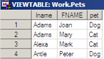
proc sort data=pets;

   by lname fname;

   run;

proc sort data=advrpt.demog(keep=subject lname fname symp)

          out=demogsymp;

   by lname fname;

   run;

data petsymptoms;

   merge pets(keep=lname fname pet)

         demogsymp(keep=subject lname fname symp);

   by lname fname;

   run;

Before performing the merge both data sets are sorted; however, the DATA step fails and the errors include a “not properly sorted” message.

WARNING: Multiple lengths were specified for the BY variable lname by input data sets. This may cause unexpected results.

ERROR: BY variables are not properly sorted on data set WORK.DEMOGSYMP.

lname=Adams FNAME=Mary pet=Cat subject=101 SYMP=02 FIRST.lname=1 LAST.lname=0 FIRST.FNAME=1

LAST.FNAME=1 _ERROR_=1 _N_=2

NOTE: The SAS System stopped processing this step because of errors.

data petsymptoms;

   length lname $10;

   merge pets(keep=lname fname pet)

         demogsymp(keep=subject lname fname symp);

^{. . . . code not shown . . . .}

In this example the truncation occurs because the length of the variable LNAME in the data set PETS ($5) determines the length for LNAME on the PDV. The result is truncation when values from DEMOGSYMP are read. In fact, because of the truncation of LNAME in the data set DEMOGSYMP, Joan Adamson becomes Joan Adams, and since Joan Adams now follows Mary Adams the rows are no longer physically sorted. It could have been worse. If Joan Adamson had a first name alphabetically after Mary, say Tricia, Tricia Adams would have followed Mary alphabetically and no sort error would have been reported.

The truncation problem could have been avoided with the use of a LENGTH statement prior to the MERGE statement (the length of LNAME on DEMOGSYMP is $10). This problem would have also been solved by simply reordering the two data sets on the MERGE statement.

Numeric BY Variables

data similar;

x = 1;

y =  3.000000000000001/3;

if x=y then put 'the same';

put x= best32.;

put y= best32.;

put x= hex16.;

put y= hex16.;

run;

Extreme care must be taken if you ever need to use numeric BY variables, especially variables with non-integer values. Because of the way that numbers are stored within the computer, even numbers that appear to be integers may not actually be integers. This can be simply demonstrated by creating a value that is slightly different from 1.

x=1

y=1

x=3FF0000000000000

y=3FF0000000000001

Examining the LOG shows that even the BEST32. format displays this value (Y=) as 1. The HEX16. format does show these two numbers differently, but really how often would you use the HEX format to double-check the integers? Worse if we were to use this variable as a BY variable as is done next, the difference is sufficient to sabotage the merge. The LOG shows that the data set BOTH has two observations—one for each value of Y, where there would only have been one observation if the values were seen as equal.

data other;

  y=1; a='a';

  run;

data both;

  merge similar

        other;

  by y;

  run;

NOTE: There were 1 observations read from the data set WORK.SIMILAR.

NOTE: There were 1 observations read from the data set WORK.OTHER.

NOTE: The data set WORK.BOTH has 2 observations and 3 variables.

At some point the fuzz rules come into play and the difference is so small that SAS considers them to be equal. In this example adding one more zero to the number of decimal places in the first definition of Y would have been sufficient for the merge to have been successful.

The take-away point is, be very careful when using numeric BY variables in a merge.

3.7.2 Variables in Common That Are Not in the BY List

After a merge or join, variables common to more than one data set will appear only once in the new data set. This means that there can be variables that overwrite each other.

In the following example we merge two data sets by SUBJECT. Each also contains the variable DATE; however, DATE is not included on the BY statement. In order to make the example a bit easier to follow the SORT steps have used the NODUPKEY option so that each SUBJECT appears only once.

proc sort data=advrpt.lab_chemistry(keep=subject labdt

                                    rename=(labdt=date))

          out=labchem nodupkey;

   by subject;

   run;

proc sort data=advrpt.ae(keep=subject aestdt

                         rename=(aestdt=date))

          out=ae nodupkey;

   by subject;

   run;

data aelab;

   merge labchem(where=(date<'01sep2006'd))

ae;

   by subject;

   run;

3.7.2 Variables in Common

Obs    SUBJECT          date

  1      200      07/28/2006

  2      201      07/06/2006

  3      202               .

  4      203      09/13/2006

  5      204      09/27/2006

. . . . portions of the table not shown . . . .

For this example the date variables have both been renamed to DATE, and then sorted by subject using the NODUPKEY option.

A WHERE clause restricting the DATE has been placed on the LABCHEM data; however, the clause does not change the resultant table.

Inspection of the data set AELAB shows that although we have restricted lab dates to those before '01sep2006'd, we seem to have dates that do not meet the criteria. In fact these are actually the AE start dates that have overwritten the dates from the LABCHEM data set. SUBJECT 202 in the LABCHEM data set has a date of '07jul2006'd, but that value has been replaced by the one in AE, which is missing.

Because the PDV is constructed from left to right, the LABCHEM date label is used in the new data set. It is also because the data are read from the rightmost data set last that the AE date overwrites the LABCHEM date.

3.7.3 Repeating BY Variables

When merging, the BY variables should identify down to the row level in all, but at most one of the data sets named on the MERGE statement. This means that at most only one of the incoming data sets will not have a sufficient key (BY variables do not identify down to the row level). When the BY variables do not form a primary key (identify down to the row level) for more than one data set, a NOTE is issued to the LOG, and more importantly, within the BY group the merge takes place as a one-to-one merge and this is rarely desirable.

NOTE: MERGE statement has more than one data set with repeats of BY values.

Here the LABCHEM and AE data sets are merged BY SUBJECT. For SUBJECT 200 there are 14 LABCHEM observations, but only 4 AE observations. The fourth AE observation is repeated for the remaining LABCHEM observations. Clearly this will be unacceptable in virtually all situations. It is essential that you understand the data and whether or not the BY variables form a sufficient key.

data aelab;

   merge labchem

ae;

   by subject;

   run;

Obs SUBJECT VISIT       LABDT  AEDESC

  1   200      1   07/06/2006  DIARRHEA (X1)

  2   200      2   07/13/2006  PAIN-NECK

  3   200      1   07/06/2006  PAIN-MUSCULAR CHEST

  4   200      4   07/13/2006  INCREASED EOS (6)

  5   200      4   07/13/2006  INCREASED EOS (6)

  6   200      5   07/21/2006  INCREASED EOS (6)

  7   200      6   07/29/2006  INCREASED EOS (6)

. . . . portions of the table are not shown . . . .

3.7.4 Merging without a Clear Key (Fuzzy Merge)

When a clear set of BY variables are not available (as was the case in the example in Section 3.7.3) logic will be needed to create the appropriate assignments. For this reason these types of merges are collectively known as fuzzy merges.

As a general rule these types of merges are best handled with an SQL step rather than the DATA step. The SQL join holds all combinations of the rows from both tables in memory (Cartesian product). This allows the programmer to apply logic to select the appropriate rows.

proc sql noprint;

create table aelab as

   select a.subject,labdt, visit, aestdt, aedesc

      from labchem as L, ae as a

         where (l.subject=a.subject)

             & (labdt le aestdt le labdt+5)

quit;

In this example we would like to identify all the adverse events for each patient that occurred within 5 days of a laboratory visit date. The subject numbers are equated in the WHERE clause as is the logic needed to evaluate the proximity of the two dates.

The DATA step can also be used to perform a fuzzy merge. In Section 6.4 a DATA step with two SET statements performs a merge. A similar technique can be applied to a fuzzy merge through logic; however, the coding can become quite tricky.

3.8 More on the SET Statement

Although a majority of DATA steps use the SET statement, few programmers take advantage of its full potential. The SET statement has options that can be used to control how the data are to be read.

END=	used to detect the last observation from the incoming data set(s) (see Section 3.9.1).
KEY=	specifies an index to be used when reading (see Section 6.6.2).
INDSNAME=	used to identify the current data source (see Section 3.8.2).
NOBS=	number of observations (see Section 3.8.1).
OPEN=	determines when to open a data set.
POINT=	designates the next observation to read (see Section 3.8.1).
UNIQUE	used with KEY= to read from the top of the index (see Section 6.6.2).

MORE INFORMATION

Several of these options are also used in the examples in Section 3.9.

3.8.1 Using the NOBS= and POINT= Options

The SET statement by default performs a sequential read; that is, one observation after another; first observation to last. It is also possible to perform a non-sequential read using the POINT= option to tell the SET statement which observation to read next. Very often the POINT= option is used in conjunction with the NOBS= option, which returns the number of observations in the data set at DATA step compilation.

The POINT= option identifies a temporary variable that indicates the number of the next observation to read. The NOBS= option also identifies a temporary variable, which after DATA step compilation, will hold the number of observations on the incoming data set.

data lastfew;

   if obs ge 10 then do pt =obs-9 to obs by 1;

      set sashelp.class point=pt nobs=obs;

      output lastfew;

   end;

   else put 'NOTE: Only ' obs ' observations.';

   stop;

   run;

This short example reads the last 10 observations from the incoming data set. The temporary variable OBS (defined by the NOBS= option) will hold the number of observations available to read. A DO loop with PT (defined by the POINT= option) as the index variable is then used to cycle through the last few observations.

Note the use of the STOP statement to terminate the DATA step after reading the 10 observations. Normally, when the last observation is read from the incoming data set, the DATA step is automatically terminated. The use of the POINT= option disables the DATA step’s ability to detect that it has finished reading from the incoming data set.

The POINT= option allows us to read observations in a non-sequential manner (in any order). When the value of the next observation to read is determined randomly, it is possible to draw a random subsample.

%macro rand_wo(dsn=,pcnt=0);

   * Randomly select observations from &DSN;

   data rand_wo(drop=cnt totl);

      * Calculate the number of obs to read;

      totl = ceil(&pcnt*obscnt);

      array obsno {10000} _temporary_;

      do until(cnt = totl);

         point = ceil(ranuni(0)*obscnt);

         if obsno{point} ne 1 then do;

            * This obs has not been selected before;

            set &dsn point=point nobs=obscnt;

            output;

            obsno{point}=1;

            cnt+1;

         end;

      end;

      stop;

      run;

%mend rand_wo;

%rand_wo(dsn=advrpt.demog,pcnt=.3)

The %RAND_WO macro shown here uses these two options to randomly read (without replacement) a subset of the observations from the incoming data set.

Because the user only specifies the fraction of the total number of observations, the macro must know the total number of available observations so that the subset size can be calculated. This value is stored in the temporary variable OBSCNT, which is defined on the SET statement through the use of the NOBS= option.

The total number of observations to be selected is calculated as a fraction of the total number of observations (OBSCNT). Although it may seem that the OBSCNT variable is being used before it is defined , in fact OBSCNT is established and assigned a value during DATA step compilation.

An array is used to track whether or not a given observation has already been selected. The array dimension must exceed the number of observations on the incoming data set. This version of the macro will accommodate up to 10,000 observations; however, arrays can easily handle much larger dimensions.

The variable POINT is randomly generated with an integer value that ranges from 1 to the number of observations in the data set (OBSCNT). This variable will be used to determine the next observation to be read.

A check is made against the flag in the array to determine if the selected observation has already been read. If it has not already been selected, it is then read. Using an array to store the flag is the fastest form of a look-up (see Chapter 6).

The SET statement uses the POINT= and NOBS= options to name the temporary variables. Tradition, although certainly not a necessity, often uses the variable names to be the same as the options (POINT=POINT and NOBS=NOBS).

When an observation has been selected, a flag is set in the array. This prevents the observation from being read again. Here the flag is a numeric 1 which takes 8 bytes of storage. If a character $1 flag had been used the array could have been defined as a character array and 70,000 bytes of memory could have been saved.

Whenever you use a SET statement inside of a loop, especially when using the POINT= option, the automatic detection of the last observation is disabled. Be sure to include a STOP to prevent an infinite loop.

The POINT= and NOBS= options can also be helpful when performing look-ahead or look-back reads of the data. In the following example we need to detect observations with certain thresholds and then determine if the value is aberrant by reporting the previous observation and the following two observations as well as the extreme value. Each observation is counted and the counter is used to establish the value used by POINT.

data surrounded(keep=subject visit sodium);

   set advrpt.lab_chemistry(keep=subject sodium

                            rename=(subject=sub1));

   cnt+1;

   if sodium ge 14.4 then do point=(cnt-1) to (cnt+2);

      if 1 le point le nobs then do;

         set advrpt.lab_chemistry point=point nobs=nobs;

         if sub1=subject then output surrounded;

      end;

   end;

run;

The observation is counted. CNT will determine the range of values (observation numbers) taken on by the temporary variable POINT.

If a given observation has a sodium value of 14.4 or greater we need to print the previous observation and the next two observations (up to 4 observations—within a subject).

The temporary variables POINT and NOBS are associated with the SET statement options of the same name.

This solution does not take into consideration whether or not a given observation has already been written to the data set. An array can be used to flag an observation once it has been used without adding much additional overhead. The sample program E3_8_1b.SAS contains a program that utilizes an array to allow a given observation to be printed only once.

3.8.2 Using the INDSNAME= Option

The INDSNAME= option was added to the SET statement in SAS 9.2. This option stores the name of the data set from which the current observation was read. Prior to its introduction, the IN= data set option was used to make this determination.

In this example we want to concatenate the two data sets (BOOMER and OTHERS) and we want to create a variable (GROUP) to identify the data source. Two solutions, one using IN= and the other using INDSNAME= are shown and contrasted.

data grouped1;

   set boomer(in=inboom)

       others(in=inoth);

   if inboom then group='BOOMER';

   else if inoth then group='OTHERS';

   run;

The IN= data set option (see Section 2.1 for more on data set options) names a temporary numeric variable that takes on the values of 0 or 1 depending on whether or not a given observation is from this data set.

IF-THEN/ELSE processing is used to determine the data source and to assign a value to the variable GROUP.

For large data sets the IF-THEN/ELSE can be time consuming and can be avoided altogether by using the INDSNAME= SET statement option.

data grouped2;

   set boomer

       others indsname=dsn;

   length group $6;

   group=scan(dsn,2,'.'),

   run;

The INDSNAME= option identifies a temporary character variable (DSN) that holds the name of the data set from which the current observation has been read.

Since the variable DSN will contain a two-level name (‘WORK.BOOMER’), the libref portion is removed using the SCAN function, and the name portion (the second word) is stored in the variable GROUP.

The length of the GROUP variable is declared; otherwise, the SCAN function would return a length of $200.

INDSNAME= has a default length of $41. This may not be long enough if you are using a physical path (which is generally not recommended by this author).

3.8.3 A Comment on the END= Option

The END= option can be used to create a numeric (0/1) temporary variable that indicates that the last record has been read. In the following example the EOF variable , which has been defined using the END=option, is used to control when a PUT statement is to be executed.

data a;

  if eof then put total=;

  set sashelp.class end=eof;

  end=eof;

  total+age;

  put 'last ' age= total= eof=;

  run;

The IF statement is true only once, and its action (the PUT statement) is executed only on the last pass of the DATA step.

last Age=12 total=212 eof=0

last Age=15 total=227 eof=0

last Age=11 total=238 eof=0

last Age=15 total=253 eof=1

total=253

However notice that the IF statement is before the SET statement. This reminds us that by default the DATA step is not fully terminated until the attempt is made to execute the SET statement after the last observation has been read.

3.8.4 DATA Steps with Two SET Statements

As can be seen in numerous examples throughout this chapter, the DATA step may contain multiple SET statements. Multiple SET statements can give you a great deal of power and flexibility over the process of reading the data. However, as you take control of the read process, exercise caution and be sure that you understand what you are requesting the DATA step to execute.

data new;

   set a;

   set b;

   run;

This simplest case of a double SET statement is essentially a one-to-one merge with restrictions. And the restrictions (conditions if you will) are very important.

Without other controls (usually supplied by the programmer), the number of observations in the new data set is determined by the number of observations in the smallest original data set. As soon as SAS reads the last observation from either data set the full DATA step is not fully executed again. You will notice that in all of the other examples with two SET statements, that there are some restrictions or controls on how the SET statements are executed. Generally we want the step to terminate on our conditions, and not necessarily just because a last observation is read from one of the data sets.

Like in a MERGE, if there are variables in common, the values that are read in from the last data set replace those read in from earlier ones. Also like in a MERGE the PDV will contain all variables from either of the incoming data sets and each variable will be assigned attributes based on its first encounter during the compilation of the DATA step. As always any variable that is read from an incoming data set is automatically retained.

As was seen in Sections 3.1.5, 3.1.6, and 3.8.1, it is possible and sometimes even very advantageous to be able to use multiple SET statements. Just be sure that you understand what is happening when you do so, and be sure that you exercise caution as you take control of the read process.

MORE INFORMATION

Two SET statements are used in the second example of Section 3.8.1. The example in Section 3.6.2 uses DOW loops to read two data sets using two SET statements.

3.9 Doing More with DO Loops

The four principle forms of the DO statement are well known and commonly applied to great advantage. However, there is so much more that we can do with this statement and sometimes in surprising ways. This section discusses a few of these techniques.

3.9.1 Using the DOW Loop

While it may have been first proposed by Don Henderson, the DOW loop, which is also known as the DO-W loop, was named for Ian Whitlock who popularized the technique and was one of the first to demonstrate its efficiencies. The DOW loop can often be used to improve DATA step performance, and in its simplest form the DOW loop takes control of the DATA step’s implied loop.

data implied;

   set big;

   output implied;

   run;

Consider the DATA step’s implied loop. During the execution phase each executable statement in the DATA step will execute once for each observation in the incoming data set (WORK.BIG). This includes a fair amount of behind the scenes processing. When the DATA statement is executed, values of derived variables are cleared and the value of the temporary variable _N_ is incremented. For the step shown here, we do not care about these things. By using the DOW loop to circumvent the implied

loop, these operations, and others, do not take place.

data dowloop;

   do until(eof);

      set big end=eof;

      output dowloop;

   end;

   stop;

   run;

To create a DOW loop place the SET statement within the control of a DO loop . Then take control of the reading process. Here the END= option is used to detect the end of file; this is used to terminate the DO UNTIL loop. When the loop terminates, we have read all the data and we are ready to terminate the DATA step. The STOP statement prevents the execution of another iteration of the implied loop .

Another typical use of a DOW loop is seen when using multiple SET statements to merge data sets. Here the mean weight of the individuals in the study is calculated and then used to determine the percent difference from the mean. Since the mean weight is calculated in a separate step, the means must be merged back onto the original data.

proc summary data=advrpt.demog;

   var wt;

   output out=means mean=/autoname;

   run;

data Diff1;

   if _n_=1 then set means(keep=wt_mean);

   set advrpt.demog(keep=lname fname wt);

   diff = (wt-wt_mean)/wt_mean;

   run;

A common solution is to use an IF statement to conditionally execute the first SET statement . Since _n_=1 will only be true once, the single observation from WORK.MEANS will only be read once. The implied loop of the DATA step will then be used to read all the observations from the analysis data set . This solution requires that the IF statement be checked for every incoming observation of the analysis data set . This is unnecessary and could be very time consuming. A DOW loop can be employed to remove the IF statement and to improve the processing efficiency of the step.

Since only one pass is made through the DATA step, the IF, which was used to control the read of the summary data set, is not needed .

data Diff2;

   set means(keep=wt_mean);

   do until(eof);

      set advrpt.demog(keep=lname fname wt)

          end=eof;

      diff = (wt-wt_mean)/wt_mean;

      output diff2;

   end;

   stop;

   run;

A DOW loop, which will execute for each observation on the analysis data set, is initiated using a DO UNTIL loop.

The END= SET statement option is used to create an end of file flag that will terminate the DO UNTIL loop .

The STOP statement terminates the DATA step with only one pass of the implied loop.

MORE INFORMATION

A DOW loop is used in Section 2.9.5 to load a hash object.

3.9.2 Compound Loop Specifications

The iterative DO loop is commonly used to step through a list of values. What is less commonly known is that we are not restricted to a single list. Here the variable COUNT takes on the values of 1, 2, 3, 5, 10, 15, 20, 26, and 33. This DO statement actually has four distinct loop specifications. The first (1 to 3) has an implied BY and the last two consist of a single value. In fact the TO and the BY are not required as is demonstrated by the last two specifications. The numbers themselves do not need to be numeric constants, but can also be stated as expressions that resolve to a number.

do count=1 to 3, 5 to 20 by 5, 26, 33;

To illustrate the use of expressions this example includes an expression; however, the iterative DO is limited to a single index variable. In the DO statement shown here, the writer would like to iterate across COUNT (1, 2, 3) and then across CNT (4, 6, 8). However this is not what happens.

do count=1 to 3, cnt=4 to 8 by 2;

The CNT=4 is interpreted as a logical expression which will resolve to 0 or 1. If CNT is not equal to 4 the second loop specification will cause COUNT to take on the values of 0, 2, 4, 6, 8; otherwise, the specification results in the values 1, 3, 5, 7. Effectively the DO statement is coded as if parentheses surrounded the expression.

do count=1 to 3, (cnt=4) to 8 by 2;

do month = 'Jan', 'Feb', 'Mar';

Since the individual values are expressions, you may also use expressions that resolve to character values.

3.9.3 Special Forms of Loop Specifications

Iterative DO loops are evaluated at the bottom of the loop. After each pass, at the END statement, the loop counter is incremented and then evaluated. This is shown in the following simple loop.

data _null_;

   do count=1 to 3;

      put 'In loop ' count=;

   end;

   put 'Out of loop ' count=;

   run;

In loop count=1

In loop count=2

In loop count=3

Out of loop count=4

The LOG shows that the variable has been incremented to 4 before it exits the loop.

Usually this behavior is acceptable; however, we may want to control whether or not the counter will be incremented the final time. We can add an UNTIL to the DO statement to provide additional control over how the loop is exited. The LOG shows that the UNTIL clause is executed before the counter (COUNT) is incremented.

data _null_;

   do count=1 to 3 until(count=3);

      put 'In loop ' count=;

   end;

   put 'Out of loop ' count=;

   run;

In loop count=1

In loop count=2

In loop count=3

Out of loop count=3

A variation on the use of the UNTIL can also be seen in the following example which counts the number of visits within clinics (CLINNUM). PROC FREQ could also have been used and would have probably been more efficient, but that is quite beside the point.

data frq;

   set demog;

   by clinnum;

   if first.clinnum then cnt=0;

   cnt+1;

   if last.clinnum then output frq;

   run;

A common approach to this type of counting problem is to use FIRST. and LAST. processing to detect the group (clinic number) boundaries. This solution requires us to track and maintain the counter (CNT) and to control the process with two IF statements. We can simplify the code and increase efficiencies by taking advantage of DO loops.

data frq;

   do cnt = 1 by 1 until(last.clinnum);

      set demog;

      by clinnum;

   end;

   run;

The DO loop surrounds the SET statement (see more about DOW loops in Section 3.9.1), and the UNTIL is used to terminate the loop. Since we do not know the upper bound of the loop, notice that the iterative portion of the loop specification (cnt=1 by 1) does not contain a TO keyword, which effectively creates an infinite loop. The loop is terminated with the UNTIL. A side benefit of this approach is that the counter variable, CNT, is automatically taken care of for us. By using the DOW loop and by eliminating the IF statements, this DATA step will execute more quickly than the first approach.

3.9.3 Special Loop Specifications

Obs    cnt    clinnum

  1     2     011234

  2     2     014321

  3     3     023910

  4     4     024477

  5     2     026789

  6     4     031234

. . . . portions of the table are not shown . . . .

3.10 More on Arrays

Arrays have been included in examples in a number of sections in this book. While their use generally seems fairly straightforward, there are a number of aspects of their definition and application that are not as generally well known.

3.10.1 Array Syntax

array chem {3} potassium sodium chloride;

The ARRAY statement gives us a way to address a list of values using a numeric index. The most common array syntax uses a list of variables. However, there are a number of alternative forms, some of which can have surprising consequences.

ARRAY Statement Syntax	Comments About This Syntax
array list {3} aa bb cc;	Array dimension of 3, indexed from 1 to 3, LIST{2} addresses BB
array list {1:3} aa bb cc;	Array dimension of 3, indexed from 1 to 3, LIST{2} addresses BB
array list {0:2} aa bb cc;	Array dimension of 3, indexed from 0 to 2, LIST{1} addresses BB (see Section 3.1.7)
array vis {16} visit1-visit16;	Undefined variables within the list will be added to the PDV
array vis {*} visit1-visit16;	SAS determines the dimension of the array by counting the elements. Variables are created as needed before the array dimension is determined.
array visit {16} ;	Will create variables VISIT1-VISIT16
array nvar {*} _numeric_;	Array includes all numeric variables in PDV order
array nvar {*} _character_;	Array includes all character variables in PDV order
array clist {3} $2 aa bb cc;	Array elements are character with a length of 2
array clist {3} $1 (‘a’, ‘b’,’c’); array clist {4:6} $1 (‘a’, ‘b’,’c’);	The variables CLIST1-CLIST3 will be created and loaded with the values of ‘a’, ‘b’, ‘c’ respectively

3.10.2 Temporary Arrays

Each of the examples of ARRAY statements in Section 3.10.1 worked with a list of variables. If the variables did not already exist the ARRAY statement would create them. Sometimes, however, you want to be able to have access to the power of an array without creating variables. Temporary arrays create unnamed, temporary, but addressable, variables that will be retained during the processing of the DATA step. Because these variables are temporary they will not be written to the new data set.

Temporary arrays are defined using the keyword _TEMPORARY_ instead of the list of variables. When using _TEMPORARY_ you must provide the array dimension.

ARRAY Statement Syntax	Comments About This Syntax
array visdate {16} _temporary_;	Values are initialized to numeric missing
array list {5} _temporary_ (11,12,13,14,15);	LIST{3} is initialized to 13
array list {5} _temporary_ (11:15);	LIST{3} is initialized to 13
array list {6} _temporary_ (6*3);	All array values are initialized to 3
array list {6} _temporary_ (2*1:3);	LIST{3} is initialized to 3, LIST{4} is initialized to 1

MORE INFORMATION

A temporary array is used in Section 3.1.2.

3.10.3 Functions Used with Arrays

Most functions will accept array values as arguments; however, some functions are designed to work with arrays, and others have particular use with arrays. Some of these functions have been shown in other sections of the book as well as here.

The DIM Function

The DIM function (introduced in Section 3.6.6) returns the dimension of an array. It is especially useful when the programmer does not know the dimension of the array when writing the program.

data newchem(drop=i);

   set advrpt.lab_chemistry

          (drop=visit labdt);

   array chem {*} _numeric_;

   do i=1 to dim(chem);

      chem{i} = chem{i}/100;

   end;

   run;

In this example we want to divide each of the chemistry values by 100. We select all numeric variables by using the _NUMERIC_ shortcut, but we do not necessarily know how many numeric variables there are in the list.

The upper bound of the iterative DO loop is specified using the DIM function. The dimension is established during the compilation of the DATA step and is available to the DIM function during DATA step execution.

The LBOUND and HBOUND Functions

The LBOUND and HBOUND functions can be especially helpful when you want to step through the elements of an array whose index does not start at one. This type of indexing is often done when the index value itself has meaning or is stored as a part of the data.

In this example we would like to find for any given subject all the other subjects that are within one inch of having the same height. This particular solution uses two passes of the data and DOW loops.

data CloseHT;

array heights {200:276} _temporary_;

do until(done);

   set advrpt.demog(keep=subject ht) end=done;

   heights(subject)=ht;

end;

done=0;

do until(done);

   set advrpt.demog(keep=subject ht) end=done;

   do Hsubj = lbound(heights) to hbound(heights);

      closeHT = heights{hsubj};

      if (ht-1 le closeht le ht+1)

          & (subject ne hsubj) then output closeHT;

   end;

end;

stop;

run;

The array is specified using the lowest and highest subject numbers.

The height for this subject is loaded into the array. Parentheses are used here; however, I suggest that curly braces should always be used for array calls.

The iterative DO loop steps through the subject numbers based on the range definition in the ARRAY statement .

The height for the other subject (HSUBJ) is recovered from the array.

The two height values are compared for proximity.

The STOP is not really needed here, but is included as a visual reminder to the programmer that we are controlling the data read using DOW loops.

Normally a code such as SUBJECT would be stored as a character field; however, storing it as a numeric field, as is done in ADVRPT.DEMOG, allows for its use as an array index.

Other Handy Functions

A number of functions that were not necessarily designed to be used with arrays also have utility when processing across arrays. The WHICHN (see Section 3.6.6) and VNAME (see Section 3.6.5) functions, and the CALL MISSING (see Sections 2.9.5 and 2.10.4) routine are particularly helpful.

These three functions are used together in this example, which compares a given visit date with all the previous visit dates with the aim of detecting duplicate visit dates. The name of the duplicate visit is returned.

data dupdates(keep=subject visit labdt dupvisit);

   array vdates {16} visit1-visit16;

   set advrpt.lab_chemistry;

   by subject;

   retain visit1-visit16 .;

   length dupvisit $7;

   if first.subject then

                  call missing(of vdates{*});

   dup = whichn(labdt, of vdates{*});

   if dup then do;

      dupvisit = vname(vdates{dup});

      if dup ne visit then output dupdates;

   end;

   vdates{visit}=labdt;

   run;

The array to hold the visit dates is established. A temporary array could have been used, except we want to retrieve the variable name through the use of the VNAME function .

The values of the array variables are retained. Since this is not a temporary array the values are not automatically retained across observations.

The array is cleared (all values set to missing) through the use of the CALL MISSING routine.

WHICHN returns the number of the first duplicate date stored in the array (the date of the current visit has not yet been added to the array).

The name of the DUP^th array element is returned. In this example the array index starts at one; consequently, the visit number and the index number are the same. VNAME would be especially needed when this was not the case.

The current visit date is added to the array.

3.10.4 Implicit Arrays

Implicit arrays (sometimes incorrectly referred to as non-indexed arrays) have been in the SAS language longer than the more recent explicitly indexed arrays. The implicit arrays utilize an implicit index – one that is not generally specified by the user. Array calls do not include an index, and consequently, the array calls can be easily confused with variable names. Most SAS programmers, including this author, try to avoid the use of implicit arrays.

This type of array was only documented through SAS 6, and then only for backward compatibility. They were completely deprecated starting with SAS 7 and are no longer supported.

Table of Contents for Chapter 3 Just In the DATA Step

Create new playlist

Sign In

Sign Up

Chapter 3 Just In the DATA Step

SEE ALSO

3.1 Working across Observations

SEE ALSO

3.1.1 BY-Group Processing—Using FIRST. and LAST. Processing

3.1.2 Transposing to ARRAYs

3.1.3 Using the LAG Function

SEE ALSO

3.1.4 Look-Ahead Using a MERGE Statement

MORE INFORMATION

SEE ALSO

3.1.5 Look-Ahead Using a Double SET Statement

MORE INFORMATION

3.1.6 Look-Back Using a Double SET Statement

MORE INFORMATION

SEE ALSO

3.1.7 Building a FIFO Stack

MORE INFORMATION

3.1.8 A Bit on the SUM Statement

MORE INFORMATION

3.2 Calculating a Person’s Age

SEE ALSO

3.2.1 Simple Formula

3.2.2 Using Functions

Caveat for YRDIF with a Basis of ACTUAL

Starting with SAS 9.3

SEE ALSO

3.2.3 The Way Society Measures Age

CAVEAT

MORE INFORMATION

SEE ALSO

3.3 Using DATA Step Component Objects

MORE INFORMATION

SEE ALSO

3.3.1 Declaring (Instantiating) the Object

3.3.2 Using Methods with an Object

3.3.3 Simple Sort Using the HASH Object

CAVEAT

3.3.4 Stepping through a Hash Table

Using the FIND Method with Successive Key Values

Using the Hash Iterator Object

3.3.5 Breaking Up a Data Set into Multiple Data Sets

MORE INFORMATION

SEE ALSO

3.3.6 Hash Tables That Reference Hash Tables

SEE ALSO

3.3.7 Using a Hash Table to Update a Master Data Set

SEE ALSO

3.4 Doing More with the INTNX and INTCK Functions

SEE ALSO

3.4.1 Interval Multipliers

MORE INFORMATION

3.4.2 Shift Operators

3.4.3 Alignment Options

Alignment with the INTNX Function

Alignment with the INTCK Function

3.4.4 Automatic Dates

Collapsing Dates

Expanding Dates

Date Intervals or Ranges

Previous Month by Name

MORE INFORMATION

SEE ALSO

3.5 Variable Conversions

3.5.1 Using the PUT and INPUT Functions

MORE INFORMATION

Character to Numeric

SEE ALSO

Numeric to Character

Using User-Defined INFORMATS

Execution or Run-Time Versions

MORE INFORMATION

SEE ALSO

Using the PUTN Function with the %SYSFUNC Macro Function

3.5.2 Decimal, Hexadecimal, and Binary Number Conversions

3.6 DATA Step Functions

Table of Contents for
Chapter 3 Just In the DATA Step

Chapter `3` Just In the DATA Step