A number of Base SAS procedures provide a variety of analysis and summarization techniques. Although some have similar capabilities, each also has some unique features. Some of these features rely on newer options or less commonly used statements. Some of these options and statements are discussed in this chapter.

MORE INFORMATION

The MEANS and SUMMARY procedures are discussed in Chapter 7.

8.1 Expanding PROC TABULATE

PROC TABULATE has been confounding new users of the procedure for a number of years. Actually it is not just new users, but any user who is new to TABULATE. For the most part, this is because the TABLE statement, which is the procedure’s primary statement, is constructed differently than any other procedure statement. Understanding the structure of the TABLE statement is the key to successfully writing a TABULATE step. Fortunately the building blocks that form the primary syntax structure of the TABLE statement are not that difficult to master. Once the fundamentals are understood, the more complex topics can be tackled more successfully.

8.1.1 What You Need to Know to Get Started

Like most procedures, PROC TABULATE has a number of statements that define how the procedure is to summarize the data. Of these statements, virtually every TABULATE step will have the following three:

CLASS	variables used to form groups within either rows or columns
VAR	numeric variables that are to be summarized
TABLE	table definition

The TABLE statement is the heart of the TABULATE step. It is the complexity of the TABLE statement that tends to thwart the user who is new to the procedure. The key to its use is to remember that it has parts (dimensions) and definitions within those parts. Break it down a piece at a time and it should make more sense.

The first and primary building blocks of the TABLE statement are the table dimensions. The table(s) generated by TABULATE can have up to three comma-separated dimensions to their definition: page, row, and column. These dimensions always appear in page, row, column order:

page	defines how the individual pages are formed (used less often)
row	defines the rows of the table within each page (almost always present)
column	defines the columns within rows and pages (always present)

You will always have at least a column dimension and you cannot have a page dimension without also having both row and column dimensions. The general makeup of the TABLE statement therefore looks something like the following. It is very important to notice that the three dimensions are comma separated. This is the only time that commas are used in the TABLE statement; the commas separate these three dimensions (definition parts).

    table page, row, column;

Generally you will want your entire table on one page; it’s easier to read, so there will not be a page dimension and your TABLE statement looks like:

    table row, column;

To build the individual page, row, and column dimensions, you will use a combination of option and element phrasing. The three types of phrases are:

singular	used when a single element is needed
concatenated	multiple elements are joined using a space
nested	one element is nested within another using an asterisk

There are several symbols or operators that are commonly used to work with these various elements. These include the following:

Operator	What It Does
space	Forms concatenations
*	Nests elements—forms hierarchies
( )	Forms groups of elements
‘text’	Adds text
F=	Assigns a format

Singular Elements

A singular element has, as the name implies, a single variable. In the following table statement there is a single classification variable (RACE) in the row dimension and a single analysis variable (WT) in the column dimension.

Since RACE is a classification variable, the resulting table will have a single row for each unique value of RACE.

ods pdf file="&path
esultsE8_1_1a.pdf"

        style=journal;

title1 '8.1.1a Proc Tabulate Introduction';

title2 'Singular Table';

proc tabulate data=advrpt.demog;

   class race;

   var wt;

   table race,wt;

   run;

ods pdf close;

image shown here

The analysis variable, WT, is specified in the VAR statement, and a single column, with a heading showing the variable’s label, will be generated for the statistic based on WT.

Since no statistic was specifically requested, the default statistic (SUM) is displayed.

Concatenated Elements

Concatenated tables allow us to easily combine multiple elements within columns and/or rows. A concatenated definition is formed when two or more space separated elements are included in the same dimension.

This example augments the table from the previous example (8.1.1a) by adding a second classification variable and a second analysis variable. The label associated with each analysis variable is by default used in the column header.

proc tabulate data=advrpt.demog;

   class race sex;

   var ht wt;

   table sex race,wt ht;

   run;

image shown here

The analysis and classification variables can be used in page, row, or column dimensions.

Nested Elements

Nested definitions allow us to create tables within tables. The nested elements can be classification variables, analysis variables, statistics, options, and modifiers; and are designated as nested elements through the use of the asterisk.

In this TABLE statement, the row dimension is singular (RACE), while the column dimension has the analysis variable (WT) nested within a classification variable (SEX).

image shown here

proc tabulate data=advrpt.demog;

   class race sex;

   var wt;

   table race,sex*wt*(n mean);

   run;

Notice also that two space-separated statistics are concatenated into a group with parentheses, and then the group is nested under the analysis variable WT, which, as was mentioned, is nested within SEX.

Combinations of Elements

In most practical uses of TABULATE, the TABLE statement will contain a combination of nested and concatenated elements. These will include not only variables and statistics, but options as well. The TABULATE procedure is rich in options, and once you have started to build simple tables such as those shown above, you would be well advised to seek out more complete references to the procedure.

The following example contains additional options, and demonstrates a few of the more complex techniques that are commonly used with many of the tables generated by TABULATE.

proc tabulate data=advrpt.demog format=8.3 ;

   class race sex ;

   var wt;

   table sex  all='Across Gender' race all,

         wt*(n*f=2.0 mean*f=7.1 var median*f=6.0)

         / box='Syngen Protocol';

   keylabel mean = 'Average'

            var  = 'Variance';

   run;

An overall format is designated for the analysis cells in the table. This default format can be overwritten by associating individual formats with each statistic . Because the other statistics have specific formats, this default format is applied only to the VARIANCE in this table.

The table definition has two concatenated elements in the row dimension. The ALL keyword summarizes across the associated element. Here it creates a row that summarizes across all values of SEX. A text label can be assigned to an element by using the equal sign. Without the text label the word ‘All’ appears in the table (as it does for RACE).

image shown here

Formats can be associated with specific variables and statistics by nesting the F= option under the desired element.

There are a number of options that can be applied on the TABLE statement (following the /) for the table as a whole. The BOX= option adds text in the upper left corner of the table.

The KEYLABEL statement allows you to assign a text label to statistics and to the keyword ALL.

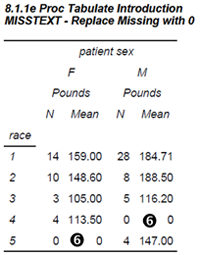
In example 8.1.1c there were no males for RACE 4 nor were there any females for RACE 5. This is reflected in missing values for the N and MEAN. Missing values can be replaced with the MISSTEXT= option .

Notice that each of the missing values has been replaced by a zero (we could have selected other text, such as an asterisk). In this example a zero for the N is appropriate; however, the mean really is not zero. We need a way to indicate that it is not a calculable value.

proc tabulate data=advrpt.demog;

   class race sex;

   var wt;

   table race,

         sex*wt='Pounds'*(n mean)

         / misstext='0' ;

   run;

image shown here

Fortunately a user-defined format can be used to provide the reader with the necessary cues.

proc format;

   value mzero

      .='----'

      other=[6.2];

   run;

proc tabulate data=advrpt.demog;

   class race sex;

   var wt;

   table race,

         sex='Gender'*wt=' '*(n mean*f=mzero.)

         /box='Weight in Pounds'

          misstext='0';

   run;

image shown here

The MZERO. format will translate a missing value into four dashes.

The MZERO. format is associated with the mean.

Since the format is applied before the MISSTEXT option, we can still use MISSTEXT=0 to replace the missing value for N.

8.1.2 Calculating Percentages Using PROC TABULATE

Because of the need to determine the denominator, the calculation of percentages in the TABULATE procedure can be problematic. Although there are situations where the determination of the denominator has to be done outside of the TABULATE step, the procedure does offer a number of tools that make this necessity less common.

PCTN and PCTSUM Options

The PCTN and PCTSUM options request the calculation of percentages based on the denominator specified using angle brackets. PCTN bases the percentages on counts (N), while PCTSUM bases the percentages on the total of an analysis variable.

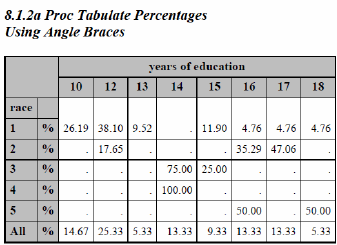
The following example requests percentages based on counts. An analysis variable (VAR statement) is not needed in this step since the percentages are based on counts and no other statistics are requested.

proc tabulate data=advrpt.demog;

   class race edu;

   table (race all)*pctn<edu>='%' ,

         edu;

   run;

Within each value of RACE, calculate the percentage of observations for each value of EDU. Since PCTN is nested within RACE, the denominator <EDU> is the total count for that value of RACE.

The column dimension is based on the classification variable EDU. There is no analysis variable; therefore, the count is converted to a percent.

Although the determination of the denominator is straightforward in this example, it is often more complex. The procedure’s documentation and Haworth (1999) show more complex examples.

image shown here

Percentage Generation Statistics

Sometimes it can be difficult to obtain the correct denominator by using the angle brackets. Fortunately there are also several percentage generation statistics. For each of these statistics, the denominator (which can be based on the report, the page, the row, or the column) is predetermined.

Percentage applies to:	Percent Frequency (N)	Percent Total (SUM)
Report	reppctn	reppctsum
Page	pagepctn	pagepctsum
Column	colpctn	colpctsum
Row	rowpctn	rowpctsum

In the following example the percentages are for the columns rather than rows. The displayed percentages are calculated using both the N (COLPCTN) and the total WT (COLPCTSUM).

proc tabulate data=advrpt.demog;

   class race;

   var wt;

   table race all,

         wt*(n colpctn mean colpctsum);

   run;

image shown here

The following example summarizes survey data. Here the response variable (RESP) takes on the values of 0 or 1 (no or yes).

proc tabulate data=survey;

   class question;

   var resp;

   table question,

         resp='responses'*(n='total responders' *f= comma7.

                           sum='total yes' *f= comma7.

                           pctsum='response rate for this question'*f=5.1

                           pctn='rate of Yes over whole survey' *f= 5.

                           mean='mean Q resp' * f=percent7.1

                           ) /rts=40;

   run;

image shown here

Notice that unlike the first example the denominator for PCTSUM and PCTN has not been specified. In this TABULATE step, the assumed denominator will be across the whole report.

The COMMA7. format has been applied to these two statistics. For the LISTING destination, the width of the format will be taken into consideration when forming the width of the column. For other destinations, such as PDF (style=minimal) which is shown here, the format width is used only in the display of the number itself and will have no affect on the column width.

8.1.3 Using the STYLE= Option with PROC TABULATE

The TABULATE procedure is one of three procedures that accept the STYLE override option. Its use in TABULATE is similar, but not the same as its use in the PRINT (see Section 8.5.2) and REPORT (see Section 8.4.6) procedures. This option allows the user to control how various aspects of the table are to appear by overriding the ODS style attributes.

Styles can be applied to a number of areas within the table from general overall attributes, down to the attributes of a specific cell. These areas include:

	Table Area	STYLE= Used on
	Box Cell	BOX= option
	Class Heading	CLASS statement
	Class Levels	CLASSLEV statement
	Analysis Variable Headings	VAR statement
	Statistics Headings (keywords)	KEYWORD statement
	Value Cells	PROC and TABLE statements
	Individual Cells	PROC and TABLE statements

To the left is a fairly typical TABULATE table. The callout numbers on the table correspond to the callout descriptions above.

image shown here

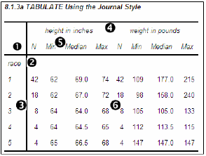
The following code was used to generate this example table. Notice that the RTS= option applies only to the LISTING destination. The ODS statements are not shown here, but are included in the sample code for this book. See http://support.sas.com/authors.

proc tabulate data=advrpt.demog;

   class race;

   var ht wt;

   table race,

         (ht wt)*(n*f=2. min*f=4. median*f=7.1 max*f=4.)

         /rts=6;

   run;

The STYLE= option can be used to control virtually all of the same attributes that can be set by the ODS style. Some of these attributes can be dependent on the ODS destination, OS, or printer; however, the most commonly used attributes are generally available. Some of these common attributes include:

Controls	Attribute	Possible Values
Font	font_face=	times, courier, other fonts supported by the OS
Text size	font_size=	6, 8, 10 (sizes appropriate to the font)
Text style	font_style=	italic, roman
Text density	font_weight=	bold, medium
Text width	font_width=	narrow, wide
Foreground color	foreground=	color (color printers or displays)
Background color	background=	color (color printers or displays)

The STYLE= option uses either curly braces or square brackets to contain the list of attributes and their values. This step demonstrates the use of the STYLE override in a variety of statements. The callout numbers refer back to the previous table, as well as to the code that follows.

proc tabulate data=advrpt.demog;

   class race / style={font_style=roman};

   classlev race / style={just=center};

   var ht wt  / style={font_weight=bold

                       font_size=4};

   table race='(encoded)',

         (ht wt)*(n*f=2.*{style={font_weight=bold

                                 font_face='times new roman'}}

                  min*f=4. median*f=7.1 max*f=4.)

         /rts=6

          box={label='Race'

               style={background=grayee}};

   keyword n / style={font_weight=bold};

   run;

The background color and a label of the RTS box are changed. Notice that the label has been removed from RACE in the TABLE statement and placed in the box using the LABEL= option.

The heading for RACE is to be written without italic (the default). For the JOURNAL style, which is used in this example, italic is the default for the heading; consequently, this option has no effect. For other styles, such as PRINTER, italic is not the default and this style override would make a difference.

The labels of the individual levels of RACE are centered. The STYLE= option on the CLASSLEV statement applies to the individual levels.

On the VAR statement the STYLE= option changes the attributes associated with the variable headings.

Adjust the label for the N statistic by bolding it. Notice that the headings for the other statistics remain unchanged.

Cell attributes associated only with the N statistic are bolded.

image shown here

8.1.4 Controlling Table Content with the CLASSDATA Option

The content of the table formed by the TABULATE procedure is influenced a great deal by the levels of classification variables in the data. Through the use of the CLASSDATA option we can identify a secondary data set to further influence the table appearance.

For the examples in this section the data set SYMPLEVELS contains only the variable SYMP, which takes on only the values ‘00’, ‘01’, and ‘02’. It should be noted, however, that in the data to be analyzed (ADVRPT.DEMOG) the variable SYMP never takes on the value ‘00’, but otherwise ranges from ‘01’ to ‘10’.

Using CLASSDATA with the EXCLUSIVE Option

The behavior and application of the CLASSDATA= option and the EXCLUSIVE option is very similar in the TABULATE step as it is in the MEANS and SUMMARY procedures (see Section 7.9). The CLASSDATA= option specifies a data set containing levels of the classification variables. These levels may or may not exist in the analysis data and can be used to either force levels into the table or to exclude levels from the table.

When the CLASSDATA= option is used with the EXCLUSIVE option, as in the following example, only those levels in the CLASSDATA= data set (including any levels not in the analysis data set) are displayed.

proc tabulate data=advrpt.demog

              classdata=symplevels exclusive;

   class symp;

   var ht wt;

   table symp,

         (ht wt)*(n*f=2. min*f=4. median*f=7.1 max*f=4.);

   run;

The symptom code ‘00’ does not exist in the analysis data, but is included in the table. Symptom codes ‘03’ through ‘10’ are excluded from the table as they do not appear in the data set SYMPLEVELS.

image shown here

When the CLASSDATA= option is used without the EXCLUSIVE option, all levels of the classification variable from either the CLASSDATA= data set or the analysis data are included in the table.

The EXCLUSIVE option can also appear on the CLASS statement; however, it will work with the CLASSDATA= option only when it is used on the PROC statement.

Using CLASSDATA without the EXCLUSIVE Option

When the EXCLUSIVE option is not used, the levels of the CLASSDATA data set can still be used to add rows to the resulting table. Here the EXCLUSIVE option has been removed from the previous example.

proc tabulate data=advrpt.demog

              classdata=symplevels;

   class symp;

   var ht wt;

   table symp,

         (ht wt)*(n*f=2. min*f=4.

                  median*f=7.1 max*f=4.);

   run;

image shown here

In this example the SYMP= ‘00’ level has been added to the table; however, no rows have been excluded.

MORE INFORMATION

Section 12.1.2 discusses the use of pre-loaded formats with PROC TABULATE to accomplish similar results.

8.1.5 Ordering Classification Level Headings

Like many procedures that use classification variables, the default order for the level headings is ORDER=INTERNAL. Unlike the REPORT procedure the default order does not change for formatted variables.

The format $SYMPTOM., which is shown here, is used with the variable SYMP. Whether or not
the format is applied, the heading values reflect the INTERNAL order of the values of SYMP. Only if the format is assigned and the ORDER=FORMATTED is specified will the headings be placed in formatted order.

proc format;

   value $SYMPTOM

      '01'='Sleepiness'

      '02'='Coughing'

      '03'='Limping'

      '04'='Bleeding'

      '05'='Weak'

      '06'='Nausea'

      '07'='Headache'

      '08'='Cramps'

      '09'='Spasms'

      '10'='Shortness of Breath';

   run;

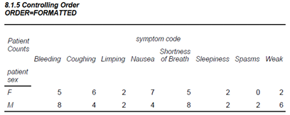
proc tabulate data=advrpt.demog

              order=formatted;

   class symp sex;

   var wt;

   table sex*wt=' '*n=' '

         ,symp

         /box='Patient Counts'

          row=float

          misstext='0';

   format symp $symptom.;

   run;

image shown here

When dealing with date values the internal order or the order of the date values is often preferred over the formatted order. In the following example the visit dates are counted within months; however, we want to view the monthly totals in chronological (INTERNAL) order. In this example if we had used either the MONNAME. or MONTH. formats, the months for the two years would have been confounded.

proc tabulate data=advrpt.lab_chemistry;

  class labdt /order=internal;

  table labdt,n*f=2.;

  format labdt monyy.;

  run;

image shown here

MORE INFORMATION

The ORDER= option is discussed in detail in Section 2.6.2. The VALUE statement in PROC FORMAT has the option NOTSORTED, which allows you to both format a variable and control the value order, is described in Section 12.4.

8.2 Expanding PROC UNIVARIATE

The capabilities of this procedure have been expanded in each of the last several releases of SAS and it is not unusual for even seasoned programmers to be only partially aware of all that it can now do. This section is a survey of some of those newer or less commonly known capabilities.

8.2.1 Generating Presentation-Quality Plots

A number of presentation-quality graphics, such as those produced by SAS/GRAPH, can also be produced by PROC UNIVARIATE. Some of the plotting capabilities require the presence of SAS/GRAPH even though a SAS/GRAPH procedure is not being called. Graphics are implemented through a series of statements which include:

HISTOGRAM	builds histograms
INSET	adds legends and text to the graph
PROBPLOT	creates probability plots
QQPLOT	creates quantile-quantile plots

The following example shows some of the flexibility of these statements by building three histograms that are overlaid by the normal distribution. In this example the plot generated by UNIVARIATE will be written to a file.

filename out821a "&path
esultsg821a.emf";

goptions device=emf

         gsfname=out821a

         noprompt;

title1 '8.2.1a Plots by PROC UNIVARIATE';

proc univariate data=advrpt.demog;

   class race sex;

   var ht;

   histogram /nrows=5 ncols=2

              intertile=1 cfill=cyan  vscale=count

              vaxislabel='Count';

   inset  mean='Mean Height: ' (5.2) / noframe position=ne

                                         height=2 font=swissxb;

   run;

   quit;

The plot is to be saved as an EMF file. EMF and the older CGM files are generally considered best if the plot is to be imported into a word processing document as it has been here. The EMF file type has the further advantage of the capability of modifying and editing the graph in the Microsoft Image Editor.

The DEVICE graphics option specifies the type of file to be created.

The GSFNAME graphics option identifies the fileref that points to the file that is to be generated.

The classification variables RACE and SEX form 10 combinations based on 5 values of RACE and 2 for SEX. These form the rows and columns for the plot.

In a color representation of the histogram, the vertical bars are cyan.

The scale of the vertical axis will be based on the patient counts. Other choices for the scale could include: PERCENT and PROPORTION.

A label is specified for the vertical axis of each of the five histograms.

The INSET statement inserts text, including various statistics, into the graph. Here the MEAN of HT is written in the upper right (NorthEast) corner of each graph using the 5.2 format and SWISSB, a SAS/GRAPH font. Notice that the default font for the title and the selected font for the INSET (SWISSB) are not particularly good choices. Under Windows most Windows fonts are available for use in graphics such as this. Alternatively the font could have been specified as font='Arial Narrow /b' . ARIAL is used in the next example.

image shown here

The histograms that are generated by the HISTOGRAM statement can be overlaid with one of several different statistical distributions. These distributions include:

normal
lognormal
gamma
Weibull

In this example a normal distribution is overlaid on a histogram of the data.

The MIDPOINTS option is used to specify both the range of the values to be plotted and the widths of the individual bins represented by the histogram bars. This MIDPOINTS option is the same as is used in PROC GCHART and the syntax is similar to an iterative DO loop.

title1 f=arial

       '8.2.1b Normal Plots by PROC UNIVARIATE';

proc univariate data=advrpt.demog;

   var wt;

   histogram /midpoints=100 to 250 by 15

              cfill=cyan vscale=count

              vaxislabel='Count'

              normal (l=2 color=red);

   inset mean='Mean: ' (6.2)/position=nw

                             height=4 font=arial;

   run;

   quit;

The normal distribution (based on the mean and variance of the data) is to be overlaid on the histogram. The line type is to be dashed (L=2) and the line color is set to RED.

The INSET statement is used to write the mean in the upper left (NorthWest) corner.

Notice the quality of the title font. The TITLE statement has specified the ARIAL font, which renders better than SWISSB in an EMF file (see Section 9.1 for more on adding options to TITLE statements).

image shown here

Although not shown in this example, you can collect the actual and predicted percentage of observations for each midpoint by using the OUTHISTOGRAM= option. This option names a data set that will contain the predicted percentage for each distribution.

Although UNIVARIATE is not a SAS/GRAPH procedure, the graphics that it produces can take advantage of some of the other SAS/GRAPH capabilities. It will recognize several SAS/GRAPH statements, including AXIS and SYMBOL statements. Additionally it respects the ANNO= option so that it can utilize the ANNOTATE facility of SAS/GRAPH.

MORE INFORMATION

Section 9.2 discusses other SAS/GRAPH options and statements that can be used outside of SAS/GRAPH. Under some conditions the default font selection for portions of the graph results in virtually unreadable text. Portions of the text in the plot in Section 8.2.1a are very hard to read. This can be mitigated by using the FTEXT option, which is also discussed in Section 9.2.

8.2.2 Using the CLASS Statement

As is the case with a number of other summary and analysis procedures, multiple CLASS statements and CLASS statement options are supported (see Section 7.1). However, unlike other summary procedures, you can only specify up to two classification variables.

One of the CLASS statement options used specifically with UNIVARIATE is the KEYLEVEL= option. This option can be used to control plot order by specifying a primary or key value for the classification variable. The selected level will be displayed first.

The single CLASS statement used here could have been rewritten as two statements, one for each classification variable.

title1 f=arial

       '8.2.2 KEYLEVEL Plots by PROC UNIVARIATE';

proc univariate data=advrpt.demog;

class race sex/keylevel=('3' 'M'),

var ht;

histogram /nrows=5 ncols=2

           intertile=1 cfill=cyan vscale=count

           vaxislabel='Count';

run;

quit;

class race / keylevel='3';

class sex  / keylevel='M';

When using a CLASS statement, the printed output is also broken up into each combination of classification variables.

In the plot, notice that RACE level ‘3’ and SEX level ‘M’ are positioned first—they have been designated as the KEYLEVELs.

image shown here

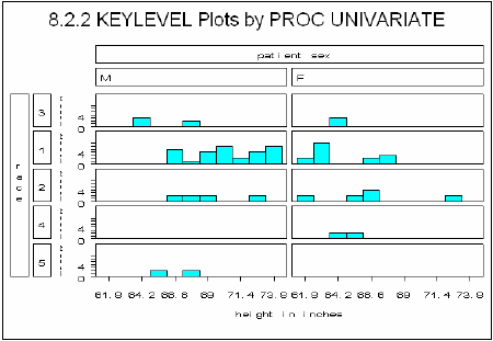
Some of the other text in this graphic is very hard to read, and not only because of the size of the graph on this page. When fonts are not explicitly declared, default hardware fonts are sometimes selected that do not render well for all devices. The FTEXT= option, which is discussed in Section 9.2, can be used to explicitly specify default fonts.

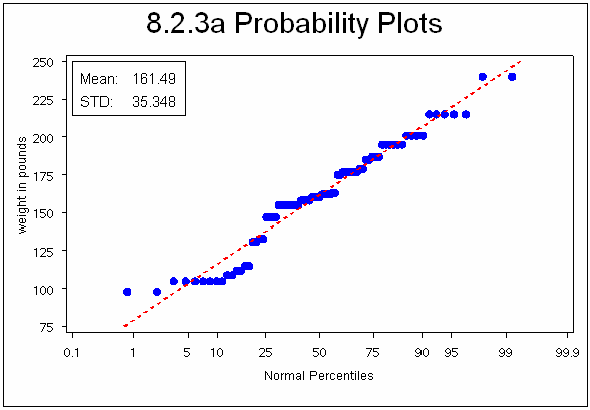
8.2.3 Probability and Quantile Plots

In addition to histograms, UNIVARIATE has the capability of generating probability and quantile-quantile plots. The syntax and resulting graphics are similar for each of these types of plots. Typically these plots are used to compare the data to a known or hypothetical distribution. Probability plots are most suited as a graphical estimation of percentiles, while the quantile-quantile plots (also known as QQplots) are better suited for the graphical estimation of distribution parameters.

Probability Plots

Probability plots can be generated by use of the PROBPLOT statement.

title1 f=arial '8.2.3a Probability Plots';

symbol1 v=dot c=blue;

proc univariate data=advrpt.demog;

   var wt;

   probplot /normal(mu=est sigma=est

                    color=red l=2 w=2);

   inset mean='Mean: ' (6.2)

         std ='STD: ' (6.3) / position=nw

                              height=4 font=arial;

   run;

The SYMBOL statement can be used to control the plot symbols for the percentiles. Here the requested plot symbol is a blue dot.

The probability plot is to be compared to a normal distribution. The mean and standard deviation can be specified (MU and SIGMA), or they can be estimated from the data, as was done here.

The estimated distribution is to be depicted with a dashed (L=2) red line with a thickness of 2.

As the distribution of the data approaches the theoretical distribution, the data percentile points should fall on the dashed line.

image shown here

QQ Plots

Rather than using the percentiles as the horizontal axis, the quantile plots break the horizontal axis into quantile ranges.

This QQPLOT statement uses the same options as were used in the percentile probability plots.

proc univariate data=advrpt.demog;

   var wt;

   qqplot /normal(mu=est sigma=est

                  color=red l=2 w=2);

   inset mean='Mean: ' (6.2)

         std ='STD: ' (6.3) / position=nw

                              height=4 font=arial;

   run;

The resulting plots are generally very similar.

image shown here

8.2.4 Using the OUTPUT Statement to Calculate Percentages

UNIVARIATE now supports the use of the OUTPUT statement. The syntax is essentially the same as is used in the MEANS and SUMMARY procedures; however, there are a number of statistics that are only available in the UNIVARIATE procedure. These statistics include several test statistics that are not included in the printed output. It is also possible to generate a wider range of percentiles. When used in conjunction with a CLASS statement, the output data set contains one observation per combination of classification levels. There are no rollup levels; the results are essentially what you would expect when using the NWAYS option with the MEANS or SUMMARY procedures.

The example shown here uses the OUTPUT statement to create a data set containing a series of percentiles that cannot be easily obtained in the MEANS or SUMMARY procedures.

proc univariate data=advrpt.demog

                noprint;

   class sex;

   var wt;

   output out=unistats

          mean = wt_mean

          pctlpre=wt_

          pctlpts=0 to 10 by 2.5,

50,

                  90 to 100 by 2.5;

   run;

The output data set will contain one observation for each level of the classification variable.

The data set UNISTATS will be created by the OUTPUT statement.

The PCTLPRE= option provides a prefix for the names of the variables containing the percentiles which are requested by the PCTLPTS option.

The percentile request uses syntax similar to an iterative DO, which can include a compound list as is shown here.

8.2.4 Using the OUTPUT Statement in UNIVARIATE

Obs sex    wt_mean  wt_0  wt_2_5 wt_5  wt_7_5 wt_10

 1   F   144.548   98    98    98   105   105

 2   M   172.913  105    105   105   105   133

Obs  wt_50 wt_90 wt_92_5 wt_95 wt_97_5 wt_100

 1    155   187    187    187    215     215

 2    177   215    215    215    240     240

8.3 Doing More with PROC FREQ

Although PROC FREQ has been a part of SAS from its inception, it has changed very little. There are, however, a few newer and underutilized options that are now available.

8.3.1 OUTPUT Statement in PROC FREQ

In addition to the ODS OUTPUT destination, the OUTPUT statement can be used in a PROC FREQ step to write statistics generated by the procedure to a data set. The list of available statistics, as is shown in the documentation, is fairly extensive and corresponds to the statistics that can be generated by the TABLES statement.

The desired statistics must be requested on the TABLES statement if they are to be available in the OUTPUT statement.

proc freq data=advrpt.demog

        (where=(race in('1','2')));

   table race*sex/chisq;

   output out=FreqStats

          all;

   run;

The CHISQ option requests a series of contingency table statistics for the table defined by RACE and SEX.

The data set WORK.FREQSTATS will be created.

Rather than select specific statistics by name, all the statistics generated by the CHISQ option on the TABLE statement are to be included in the data set. This option generates a warning as the ALL keyword requests statistics that are not included in the CHISQ option. The warning would not have been issued had either the ALL been replaced with CHISQ or if the additional statistics requested by the ALL had been included in the TABLES statement (MEASURES, CMH, N).

The portion of the table generated by the CHISQ option is shown here.

image shown here

Many of these same values can be found in the data set, which has been printed below.

8.3.1 Using the OUTPUT Statement in FREQ

Obs  N  _PCHI_ DF_PCHI  P_PCHI _LRCHI_ DF_LRCHI P_LRCHI _AJCHI_ DF_AJCHI P_AJCHI _MHCHI_

1   60  2.59259   1    0.10736 2.56359    1     0.10935 1.74934     1    0.18596 2.54938

Obs DF_MHCHI   P_MHCHI   XPL_FISH   XPR_FISH   XP2_FISH     _PHI_    _CONTGY_    _CRAMV_

1      1       0.11034   0.093531    0.97063    0.15174   -0.20787    0.20352   -0.20787

8.3.2 Using the NLEVELS Option

The NLEVELS option on the PROC FREQ statement generates a summary table that shows the number of levels, including missing, for each of the classification variables included in the TABLES statement. In this example the TABLE statement requests a count of levels for all variables in the data set. The NOPRINT option prevents the printing of all tables, except the one generated by the NLEVELS option.

proc freq data=advrpt.demog

          nlevels;

   table _all_/noprint;

   run;

The resulting table shows all the variables in ADVRPT.DEMOG and the number of distinct values of each.

image shown here

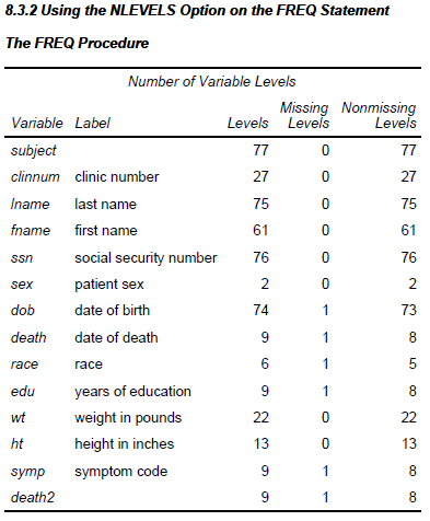
Knowing the number of distinct levels of a variable can be helpful when writing automated programs. The data contained in the NLEVELS table can be written to a data set using the ODS OUTPUT destination, and once there it can be harvested as metadata for use by the macro language.

ods output nlevels=varcnts;

proc freq data=advrpt.demog

          nlevels;

   table _all_/noprint;

   run;

MORE INFORMATION

The ODS OUTPUT destination is discussed in more detail in Section 11.1.

8.4 Using PROC REPORT to Better Advantage

Like PROC TABULATE, the REPORT procedure is underutilized by many analysts. The details of its usage can be found in Carpenter’s Complete Guide to the SAS REPORT Procedure (Carpenter, 2007a). This section will not provide an introduction to the procedure, but will instead cover a few topics that have been known to be problematic.

Much of the confusion is centered on the use of the compute block, which is unique to PROC REPORT. Consequently, most of the examples in this section involve the use of the compute block. Carpenter (2007a) has a number of more detailed examples on the syntax, use, and operating sequencing of the compute block. This book also includes a Microsoft PowerPoint copy of Russ Lavery’s “Animated Guide to the REPORT Procedure’s Compute Block.”

MORE INFORMATION

The use of pre-loaded formats with PROC REPORT to create report subsets can be found in Section 12.1.1.

8.4.1 PROC REPORT vs. PROC TABULATE

Both the REPORT and TABULATE procedures can create summary reports and each has basically the same access to the standard suite of summary statistics.

Unlike TABULATE, the REPORT procedure can provide detail reporting as well as summary reporting capabilities. REPORT has the added flexibility to calculate and display columns of information based on other columns in the report.

Because of the unique way that the TABULATE procedure structures the report table it has a great deal more flexibility to present the groups, sub-groups, and statistics as either rows or columns. This is especially true for vertically concatenated reports, which are very straightforward in TABULATE and difficult in REPORT (see Carpenter, 2007a, Section 10.1 for details on creating a vertically concatenated report using PROC REPORT).

8.4.2 Naming Report Items (Variables) in the Compute Block

Compute blocks are unique to the REPORT procedure. While they have a number of similarities to the DATA step, there are sufficient differences, not only in syntax, but more importantly in how they are executed, which is why they warrant a discussion in this book.

In the DATA step you name the items (variables) on the Program Data Vector , PDV, explicitly by name. Although the term variable is often used to address values in the compute block, they are more accurately known as report items. In the compute block the rules for naming report items are not nearly as straightforward as in the DATA step. In the compute block there is no PDV, and the compute block can be used to address report items that are not actually variables.

There are four different situations that determine how a report item is to be named in the compute block. These result in three distinct report item naming conventions.

Explicitly by Name

In the DATA step variable names are used explicitly. While this same naming convention will sometimes work in the compute block, you need to understand when it will and will not work. The name is used explicitly when the variable or report item:

has a define usage of GROUP, ORDER, COMPUTED, or DISPLAY
is a temporary variable, which is created and used only in a compute block
is the automatic temporary variable named _BREAK_
is a report item alias (see below)

Using a Compound Name

Compound variable names are needed when a report item has a define usage of ANALYSIS, which means that is has been used to calculate a statistic (SUM is the default). The compound name is a combination of the variable name and the statistic that it has been used to calculate. The general form is variablename.statistic, and in the compute block you might address the mean of the variable WT as shown to the left.

compute wt;

   wt.mean = wt.mean/2.2;

endcomp;

Directly When Using an Alias

Creating an alias of a report item allows you to use that report item in multiple ways. The following COLUMN statement generates a series of aliases for the HT analysis variable. Each of these aliases will be used to calculate a different statistic.

column region ht

        ht=htmin  ht=htmax

        ht=htmean ht=htmedian;

When an alias is used in a compute block, it is named explicitly. Here the HTMIN alias of HT is used in a LINE statement.

compute after;

   line @3 'Minimum height is ' htmin 6.1;

endcomp;

Indirectly When Using the Absolute Column Number

The define type of ACROSS creates a series of columns. These columns, and indeed any column in the report, can be referenced by using the column number as an indirect column reference.

This pseudo variable name is always of the form, _Cxx_, where the xx is the column number as read from left to right on the report. The column count even includes any columns that will ultimately not be printed, e.g., those columns defined with NOPRINT or NOZERO.

When one or more report items have a define usage of ACROSS, it is not possible to address the transposed columns by name. To address these columns it is necessary to use absolute column numbers.

MORE INFORMATION

Absolute column references are used in the example in Section 8.4.3.

8.4.3 Understanding Compute Block Execution

In the following example a compute block is used to convert the mean weight from pounds to kilograms. Since WT is nested under SEX, which has a define usage of ACROSS, there will be two columns associated with WT. As a consequence, absolute column numbers must be used in the compute block that performs the conversion .

Although this step executes without any syntax errors, it contains a huge logic error. In order to understand the error and what causes it we need to first understand the execution of the compute blocks.

proc report data=advrpt.demog nowd;

   column edu sex,wt  wt=allwtmean;

   define edu / group 'Years/Ed.';

   define sex / across order=formatted;

   define wt  / mean 'Mean' format=5.1;

   define allwtmean / mean 'Mean' format=5.1;

   compute wt;

      _c2_ = _c2_/2.2;

      _c3_ = _c3_/2.2;

   endcomp;

   compute allwtmean;

      allwtmean = allwtmean/2.2;

   endcomp;

run;

Patient weight is nested within SEX, which has a define usage of ACROSS. An alias for WT, ALLWTMEAN, is also declared.

In the compute block for WT, the values for each of the two genders are converted from pounds to kilograms.

_C2_ holds the mean weight of female patients and is the second column in the report (counting from left to right).

ALLWTMEAN (mean weight ignoring SEX) is a computed report item and is named directly.

In this example there are two compute blocks, one associated with WT and one for the alias ALLWTMEAN. Since there are two columns associated with WT within SEX (one for each of the two genders), the compute block for WT will execute twice for each row in the report. As a matter of fact, counting the one for ALLWTMEAN, three compute block executions take place for each report row.

8.4.3a Showing ACROSS With Compute Blocks

Convert LB to KG

        patient sex

 Years      F      M

   Ed.   Mean   Mean   Mean

    10     .    88.2   88.2

    12   31.4   81.7   76.4

    13   44.4   86.8   89.5

    14   22.7   47.7   49.1

    15   34.0   60.5   70.7

    16   32.6   75.9   75.1

    17   29.5   70.5   66.0

    18     .    79.1   79.1

Since the compute block for WT will execute twice for each report row, this causes a very nasty error. Notice that in the mean weights for females, the values have been divided by 2.2 twice. The problem goes away if the calculations for _C2_ and _C3_ are placed in the compute block for ALLWTMEAN, which is executed only once for each row.

The compute block for ALLWTMEAN will execute only once. Any given compute block can reference any report item to its left on the COLUMN statement, so there is no issue with placing references to all three columns in this single compute block.

The resulting report now shows that the mean weight for the females has been successfully converted to kilograms.

proc report data=advrpt.demog nowd;

   column edu sex,wt wt=allwtmean;

   define edu / group 'Years/Ed.';

   define sex / across order=formatted;

   define wt  / mean 'Mean' format=5.1;

   define allwtmean / mean 'Mean' format=5.1;

   compute allwtmean;

      _c2_ = _c2_/2.2;

      _c3_ = _c3_/2.2;

      allwtmean = allwtmean/2.2;

   endcomp;

run;

8.4.3b Showing ACROSS With Compute Blocks

Convert LB to KG

             patient sex

      Years      F      M

        Ed.   Mean   Mean   Mean

         10     .    88.2   88.2

         12   69.1   81.7   76.4

         13   97.7   86.8   89.5

         14   49.9   47.7   49.1

         15   74.8   60.5   70.7

         16   71.8   75.9   75.1

         17   64.9   70.5   66.0

         18     .    79.1   79.1

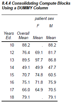
8.4.4 Using a Dummy Column to Consolidate Compute Blocks

In the previous section we were able to solve a nasty problem by taking advantage of a compute block associated with a report item that lay to the right of the columns with the problem. When there is no compute block ‘to the right’, a compute block that is based on a dummy column can be used to calculate all three mean values. In this example, ALLWTMEAN is to the left of the other columns. Consequently, its compute block could not be used in calculations of report items to its right in the COLUMN statement.

proc report data=advrpt.demog nowd;

   column edu wt=allwtmean sex,wt dummy ;

   define edu / group 'Years/Ed.';

   define allwtmean / mean 'Overall Mean' format=7.1;

   define sex / across order=formatted;

   define wt  / mean 'Mean' format=5.1;

   define dummy / computed noprint ;

   compute dummy;

      _c4_ = _c4_/2.2;

      _c3_ = _c3_/2.2;

      allwtmean = allwtmean/2.2;

   endcomp;

run;

The DUMMY column must be the furthest to the right on the COLUMN statement. Or at least it must be to the right of any columns used in the compute block.

The NOPRINT option appears on the DEFINE statement for DUMMY as we are not interested in having this column displayed.

The column numbers for the male and female values have now changed (_C3_ is now the mean weight of the females). Since these three conversions are independent of each other, they can be performed in any order.

image shown here

8.4.5 Consolidating Columns

Sometimes we want to show the information contained in multiple report items within a single column. Doing so provides us with additional control over the appearance of the report items. In the following example we want to display the mean along with its standard error, and we want the values to be displayed as mean (se).

proc report data=advrpt.demog nowd;

   column edu sex,(wt wt=wtse meanse );

   define edu    / group 'Years/Ed.';

   define sex    / across order=formatted;

   define wt     / mean noprint;

   define wtse   / stderr noprint;

   define meanse / computed 'Mean (SE)' format=$15.;

   compute meanse/char length=15;

      _c4_ = cat(put(_c2_,5.2),' (',put(_c3_,5.2),')'),

      _c7_ = cat(put(_c5_,5.2),' (',put(_c6_,5.2),')'),

   endcomp;

   run;

WT, its alias WTSE, and the computed report item MEANSE, are all nested under SEX , which has a define usage of ACROSS.

The values for WT and WTSE are not to be printed. They are used only to form the concatenated value (MEANSE).

The computed report item MEANSE is defined.

The computed variable MEANSE is defined as character with length of 15.

The mean (_C2_) and the SE (_C3_) for females are concatenated into a single value (_C4_).

The computed report item MEANSE is constructed in the compute block by concatenating the MEAN and SE, neither of which is printed individually. This also allows us to add the parentheses.

8.4.5 Consolidating Columns within an ACROSS Variable

Weight Within Gender

                       patient sex

      Years  F                M

        Ed.  Mean (SE)        Mean (SE)

         10    .   (  .  )    194.1 ( 5.75)

         12  152.0 ( 9.71)    179.8 ( 6.73)

         13  215.0 (  .  )    191.0 (12.00)

         14  109.9 ( 1.78)    105.0 ( 0.00)

         15  164.6 (13.72)    133.0 ( 0.00)

         16  158.0 ( 0.00)    167.0 ( 7.70)

         17  142.8 ( 9.84)    155.0 ( 0.00)

         18    .   (  .  )    174.0 (15.59)

Because SEX has the define usage of ACROSS, absolute column references must be used in the compute block.

8.4.6 Using the STYLE= Option with LINES

When writing to destinations such as PDF, RTF, and HTML, the STYLE= option can be used to override values in the ODS style without using PROC TEMPLATE to redefine the style itself. This option is available for use with the REPORT, TABULATE, and PRINT procedures. In REPORT, it can be used with the LINE statement in the compute block.

Here the style override option is used to change the justification, font, font style, and font size of the text written by the LINE statements.

proc report data=advrpt.demog nowd;

   column edu sex,(wt wt=wtse) wt=n wt=allwt;

   define edu / group 'Years/Ed.';

   define sex / across order=formatted;

   define wt  / mean 'Mean' F=5.1;

   define wtse / stderr 'StdErr' f=5.2;

   define n   / n noprint;

   define allwt / mean 'Overall/Mean' f=5.1;

   compute after/style(lines)={just=center

                               font_face=Arial

                               font_style=italic

                               font_size=10pt};

      line ' ';

      line @10  'Overall Statistics:';

      line @15 n 3. ' Subjects had a mean weight of '

           allwt 5.1 ' pounds';

   endcomp;

run;

In the LINE statement, the @10 and @15 control the left most starting position for the text. These values are ignored for destinations other than LISTING, and the STYLE option is ignored in the LISTING destination.

Inline formatting can also be used in the compute block with the LINE statement; however, there are a couple of things that you should be aware of as the formatting becomes more complicated. Since LINE statements are consolidated before execution, you may not be able to change style attributes at the LINE statement level within a compute block. In this example the STYLE option will be applied to each of the LINE statements.

image shown here

If you do need to change attributes on individual lines, the inline formatting will probably have to be done in a separate compute block. This can pose a problem if you are working with the COMPUTE AFTER (end of report) compute block.

In the following example an artificial variable PAGEFLAG is introduced. Since it is a constant, the COMPUTE AFTER PAGEFLAG block and the COMPUTE AFTER block will both take place at the end of the report. This will allow LINE statements with two different styles to be used.

* Show the use of the inline formatting;

ods rtf file="&path
esultsE8_4_6b.rtf";

ods escapechar='~';

title1 '8.4.6b Using Inline Formatting';

title2 '~S={just=r} Patient Weight';

data demog;

set advrpt.demog;

pageflag=1;

run;

proc report data=demog(where=(sex='F')) nowd;

   column pageflag edu sex,(wt wt=wtse) wt=n wt=allwt;

   define pageflag / group noprint;

. . . . define statements not shown . . . .

   compute after pageflag;

   line "~S={just=l background=pink } Females Only";

   endcomp;

   compute after/style(lines)={just=center

                               font_face=Arial

                               font_style=italic

                               font_size=10pt};

      line ' ';

      line @10  'Overall Statistics:';

      line @15 n 3. ' Subjects had a mean weight of '

                     allwt 5.1 ' pounds';

   endcomp;

run;

ods rtf close;

An escape character is specified for use with the inline formatting sequences.

Inline formatting is used to right justify the title.

A constant variable is created that will allow us to have a second compute block at the end of the report.

This report item is not printed, but since it has a define usage of GROUP, a compute block can be associated with it.

A COMPUTE AFTER block is defined for the constant report item.

Effectively there are now two compute blocks that will be executed at the end of the report.

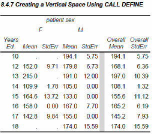
8.4.7 Setting Style Attributes with the CALL DEFINE Routine

Unique to PROC REPORT, the CALL DEFINE routine can be used in the compute block to set various attributes. Unlike the STYLE= option shown in Section 8.4.6, as a routine CALL DEFINE can be conditionally executed. This highly flexible routine can be used to set or reset a number of attributes including formats, links, and styles.

In the following example the DEFINE routine is used to form a visual boundary by changing the background color for a dummy column. The PDF destination is used to create the report, and a gray vertical band is generated through the use of a computed variable, DUMMY, and the CALL DEFINE routine.

proc report data=advrpt.demog nowd;

   column edu sex,(wt wt=wtse) dummy

          wt=allwt wt=allwtse;

   define edu / group 'Years/Ed.';

   define sex / across order=formatted;

   define wt  / mean 'Mean' F=5.1;

   define wtse / stderr 'StdErr' f=5.2;

   define dummy / computed ' ' ;

   define allwt / mean 'Overall/Mean' f=5.1;

   define allwtse / stderr 'Overall/StdErr' f=5.2;

   compute dummy/char length=1;

      call define(_col_,'style',

                        'style={background=cxd3d3d3

                                cellwidth=1mm}'),

      dummy = ' ';

   endcomp;

run;

A computed column is created to hold the visual separator.

The label for the computed column is set to blank.

_COL_ indicates that the result of the routine is to be applied to the entire column. The second argument, STYLE, indicates that this is to be a style override. The third argument is the style attribute that will be overridden.

The background color is set to a light shade of gray.

Although the cell width is set to 1mm, you will probably need to experiment to obtain the desired width as this is only a nominal value.

The computed variable is assigned a missing value.

image shown here

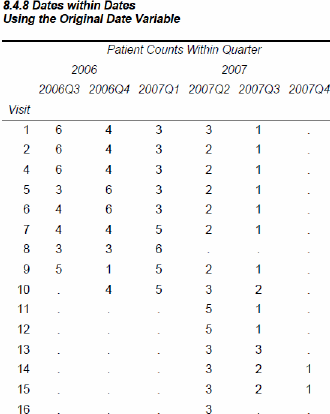
8.4.8 Dates within Dates

When a report item is nested within itself, the resulting table is generally less than satisfactory unless you take some precautions.

Processing dates can be especially problematic as they can fall into several ranges at the same time. A given date is specific to a year, to a quarter, and to a month. When you want to create summarizations for more than one date level at the same time, you could create dummy variables for each level and then summarize using these levels as classification variables. This requires an extra step, such as the one shown to the left, which we can avoid when using PROC REPORT.

data visits;

   set advrpt.lab_chemistry

      (keep=visit labdt sodium);

   year=year(labdt);

   qtr = qtr(labdt);

   run;

In the previous DATA step, the variable LABDT is used to create two different summary levels. The date is being used two different ways at the same time. You can conduct the same type of summarizations in a REPORT step by creating an alias; however, whenever you nest a variable under itself, you should be aware of some of the pitfalls of the technique.

The following report counts the number of patients that were seen for each visit type within quarter and year. The same variable, LABDT, is used for both the quarter and year summary.

proc report data=advrpt.lab_chemistry nowd;

   column visit ('Patient Counts Within Quarter'

                  labdt=year, labdt,sodium,n);

   define visit  / group'Visit';

   define year   / across format=year. order=formatted ' ' ;

   define labdt  / across format=yyq6. order=internal ' ';

   define sodium / display ' ';

   define n      / ' ' format=2. nozero

                   style={just=center};

   run;

Spanning text is defined for the report.

The lab date is nested under an alias of lab date (YEAR). The N statistic is nested under SODIUM, which is in turn nested under date.

The dates will be consolidated into each represented year. The order will be determined by the formatted value.

The quarters are nested within year, and every quarter—regardless of year—will appear under each year. This means that ‘2007Q1’ will appear without any values under year 2006. We can eliminate these empty columns through the use of the NOZERO option.

Any column that is always empty is completely eliminated by the NOZERO option.

The STYLE= option is used to center the counts within each quarter.

The use of the NOZERO option is a key technique when nesting variables such as a date within itself. Without the use of the NOZERO option there would necessarily be a number of empty columns.

This example counts the number of patients with non-missing values of SODIUM. While the N statistic can be used for the lab date, the NOZERO option will not work on a grouping variable. Consequently, an intermediate analysis variable, SODIUM, is needed. SODIUM is a variable that in this case we are not particularly interested in, but it allows us to use the N statistic.

In this example the quarters are ordered appropriately and the ORDER=INTERNAL option is not necessary. If, instead of using quarters the dates had been grouped using month name, this option could have been used to place the columns in date order rather than alphabetical order.

image shown here

8.4.9 Aligning Decimal Points

Unlike PROC PRINT the REPORT procedure does not by default align decimal points within a column of the output. This can be seen in the following example, which prints the values of SODIUM in the LAB_CHEMISTRY data set.

title1 f=arial

       '8.2.2 KEYLEVEL Plots by PROC UNIVARIATE';

proc univariate data=advrpt.demog;

class race sex/keylevel=('3' 'M'),

var ht;

histogram /nrows=5 ncols=2

           intertile=1 cfill=cyan vscale=count

           vaxislabel='Count';

run;

quit;

image shown here

There are a couple of easy ways to align the decimal points in the SODIUM column. When you are writing to the RTF or PDF destination, as we are here, the JUST= style attribute can be used on the DEFINE statement.

proc report data=advrpt.Lab_chemistry nowd;

  column subject visit labdt sodium;

  define sodium / style(column)={just=d};

  run;

ods pdf file="&path
esultse8_4_9a.pdf"

        style=journal;

title2 'Unaligned Decimals';

proc report data=advrpt.Lab_chemistry

            nowd;

   column subject visit labdt sodium;

   run;

ods pdf close;

image shown here

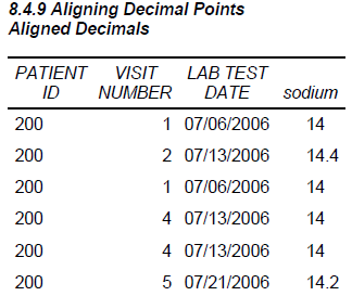
While the columns are aligned, the decimal point is not always shown. When the use of a format is an option, and it generally is, the format will not only cause the decimal points to be aligned, but the decimal point will be displayed.

Here a format is used to align the decimal points instead of the style override.

proc report data=advrpt.Lab_chemistry nowd;

  column subject visit labdt sodium;

  define sodium / f=4.1;

  run;

image shown here

8.4.10 Conditionally Executing the LINE Statement

Unlike in the DATA step where we can conditionally execute the PUT statement, the analogous LINE statement in a PROC REPORT compute block cannot be conditionally executed. However, we can conditionally assign values to write with the LINE statement. The first attempt, which is shown below, demonstrates this problem.

In this example we would like to write a message following each level of SEX. If the count is 35 or more, we want to display the mean weight; however, for counts under 35, we just want a note stating the low count.

proc report data=advrpt.demog nowd;

column sex race wt wt=meanwt;

define sex  / group;

define race / group;

define wt    / analysis n 'Patient Count';

define meanwt/ analysis mean 'Mean Weight' f=5.1;

compute after sex;

   if wt.n ge 35 then do;

      line 'Overall mean weight is: ' meanwt 5.1;

   end;

   else line 'Patient Count Below 35';

endcomp;

run;

The text will be written after each grouping of the report item SEX.

If the total N is greater than 34, we want to write the mean using a LINE statement.

For small numbers, we just want this constant text to be written.

Clearly the LINE statements have not been executed conditionally. In fact both statements have been executed for each level of the report item SEX! This is obviously not what we intended, but what actually happened?

image shown here

During the process that evaluates the statements in a compute block, the LINE statements are effectively moved to the end of the step. The compute block from above essentially becomes the one shown here. This behavior is very different from anything that we see in the DATA step.

compute after sex;

   if wt.n ge 35 then do;

   end;

   else;

   line 'Overall mean weight is: ' meanwt 5.1;

   line 'Patient Count Below 35';

endcomp;

Consequently we cannot conditionally execute the LINE statement; we can, however, conditionally build what will be displayed by the LINE statement.

compute after sex;

   if wt.n ge 35 then do;

      text= 'Overall mean weight is: '||put(meanwt,5.1);

   end;

   else text = 'Patient Count Below 35';

   line text $31.;

endcomp;

Here we create a temporary variable (TEXT) that will take on the desired value to be displayed.

The LINE statement is then executed.

image shown here

8.5 Using PROC PRINT

PROC PRINT is one of those procedures that everyone uses on a regular basis. It is designed to dump the data and is generally not used to generate pretty output. However, there are some things that you can do with PRINT that can make even this standard procedure more useful.

8.5.1 Using the ID and BY Statements Together

Although the PRINT procedure does not have a CLASS statement you can offset groups with a combination of the BY and ID statements. Variables that are common to these two statements will cause two changes to the standard report generated by PROC PRINT.

In the PRINT step to the left, both the BY and ID statements use the variable REGION. When used together this way, the value for REGION is written only once for each region (this is the default behavior for PROC REPORT for GROUP and ORDER variables). Also a blank line has been inserted after each REGION.

title1 '8.5.1 PRINT with BY and ID Statements';

proc print data=advrpt.clinicnames;

   by region;

   id region;

   var clinnum clinname;

   run;

This specialized layout for PROC PRINT is generated when all of the variables in the BY statement also appear in the same order at the start of the ID statement.

8.5.1 PRINT with BY and ID Statements

region    clinnum    clinname

  1       011234     Boston National Medical

          014321     Vermont Treatment Center

  10      107211     Portland General

          108531     Seattle Medical Complex

  2       023910     New York Metro Medical Ctr

          024477     New York General Hospital

          026789     Geneva Memorial Hospital

. . . . portions of this table are not shown . . . .

8.5.2 Using the STYLE= Option with PROC PRINT

The STYLE= option, which is discussed in Sections 8.1.3 and 8.4.6, can also be used with PROC PRINT. This is a style override option and it is used to change the attributes generated by the selected ODS style.

In the general syntax shown here, notice that the attributes are surrounded by curly brackets.

style<(location)>={attribute=attribute_value}

In the current releases of SAS you are able to use the square bracket instead of the curly braces.

Specification of the location is optional, since there is a default assignment when it is left off. However, you generally will want to specify the location as it is used to control where the attribute assignment is to be applied. Supported locations include:

DATA	cells (also COLUMNS or COL)
TOTAL	sub-total (used on the SUM statement)
GRANDTOTAL	overall total (used on the SUM statement)
HEADER	column header (also HEAD and HDR)
N	used when the N option is specified
OBS	cells in the OBS column
OBSHEADER	header for the OBS column
TABLE	controls table structure such as cell width

The STYLE= option can be applied on the PROC PRINT statement as well as on other procedure step statements. A combination of the specified location and the statement containing the option will determine what portion of the table is modified by the option.

Not all style option locations are appropriate for all PRINT statements. The following table shows the available locations and the statements to which they can be applied.

PROC Statements	Supported Style Locations
PROC PRINT	data header, n, obs, obsheader, table
BY	none
ID	header, data
VAR	header, data
SUM	header, data, total, grandtotal

Some of the style attributes that can be modified include:

BACKGROUND
BORDERCOLOR
BORDERCOLORDARK
BORDERCOLORLIGHT
FONT_FACE
FONT_WEIGHT
FOREGROUND

In the PROC Statement

When the STYLE= option is used on the PROC statement, the attributes tend to control the overall appearance of this particularly attractive table.

title1 'Using STYLE= with PRINT';

title2 '8.5.2a on the PROC Statement';

proc print data=advrpt.demog(obs=5)

      style(col)= [background=cyan]

      style(header)= [background=yellow

                      font_weight=bold]

      style(obs)= [background=pink]

      style(obsheader)= [background=cyan]

   var clinnum subject sex dob;

   run;

The background color is reset for all the data values in each column.

Two attributes for the column headers are reset.

The background color for the OBS column is set to pink.

The background color for the OBS column header is changed to CYAN.

image shown here

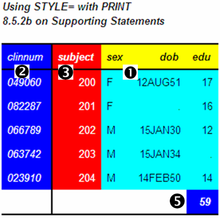
Supporting Statements

Although style attributes used with the PROC statement generally apply to the table as a whole, STYLE= options that are applied on supporting statements give you more specific control. Additionally these attributes tend to override those set on the PROC statement.

proc print data=advrpt.demog(obs=5)

      style(col)= [background=cyan]

      style(header)= [background=yellow

                      font_weight=bold]

   id clinnum / style(hdr data )={background=blue

                                 foreground=white};

   var subject / style(header)={background=red

                                foreground=white}

                 style(column)={background=red

                                foreground=white};

   var sex dob edu;

   sum edu / style(grandtotal)={font_weight=bold

                                background=blue

                                foreground=white};

   run;

Like the CLASS statement (see Section 7.1), which can be split into multiple statements, several of the PRINT statements that allow lists of variables can also be split into multiple statements. This allows you to specify different options for different variables. We can take advantage of this ability when applying the STYLE= option ➌➍.

The STYLE= options on the PROC statement override the defaults associated with the ODS style, JOURNAL.

Two locations are specified for the ID variable. Notice that the HEADER location has been abbreviated as HDR.

Two STYLE= options, each with its own location, are specified. Since both have the same attributes, they could have been combined as in .

The VAR statement has been split into two statements. These variables do not have a style override and will utilize the attributes specified in the PROC statement .

The column total receives three attribute overrides.

image shown here

MORE INFORMATION

The style override option is used to produce traffic lighting effects is discussed in Section 11.5.4.

8.5.3 Using PROC PRINT to Generate a Table of Contents

The PRINT procedure is designed to work with lists of information. When the list of values contains links to other files, PRINT can create a table of contents to a report.

In this example HTML anchor tags are formed as data values. When they are displayed by ODS in the HTML destination these values become links to other files.

data clinlinks(keep=region clinnum clinic);

   set clinicnames;

   length clinic $70;

   clinic = catt("<a href='cn",

                 clinnum,

                 ".html'>",

                 clinname,

                 "</a>");

   run;

proc print data=clinlinks;

   var region clinnum clinic;

   run;

The character variable CLINIC is used to hold the HTML anchor tag. The CATT function is used to concatenate the pieces of the anchor tag statement. The clinic number is used in the name of the file to which the tag will link. The name of the clinic will be displayed. In the PROC PRINT step all that is required is to display the data. The LISTING destination does not know what to do with an HTML anchor tag and will therefore show the data as it is stored .

8.5.3 Clinics in the Study

Obs    region    clinnum                            clinic

  1      4       049060     <a href='cn049060.html'>Atlanta General Hospital</a>

  2      6       066789     <a href='cn066789.html'>Austin Medical Hospital</a>

  3      5       051345     <a href='cn051345.html'>Battle Creek Hospital</a>

  4      3       031234     <a href='cn031234.html'>Bethesda Pioneer Hospital</a>

. . . . portions of the table are not shown . . . .

When the table is displayed using the HTML destination, the value is interpreted as an anchor tag and is displayed as a linkable item. Here the first four items in the PROC PRINT are shown.

image shown here

MORE INFORMATION

The creation of links is discussed in more detail in Section 11.4.

Table of Contents for Chapter 8 Other Reporting and Analysis Procedures

Create new playlist

Sign In

Sign Up

Chapter 8 Other Reporting and Analysis Procedures

MORE INFORMATION

SEE ALSO

8.1 Expanding PROC TABULATE

SEE ALSO

8.1.1 What You Need to Know to Get Started

Singular Elements

Concatenated Elements

Nested Elements

Combinations of Elements

8.1.2 Calculating Percentages Using PROC TABULATE

PCTN and PCTSUM Options

Percentage Generation Statistics

SEE ALSO

8.1.3 Using the STYLE= Option with PROC TABULATE

8.1.4 Controlling Table Content with the CLASSDATA Option

Using CLASSDATA with the EXCLUSIVE Option

Using CLASSDATA without the EXCLUSIVE Option

MORE INFORMATION

8.1.5 Ordering Classification Level Headings

MORE INFORMATION

SEE ALSO

8.2 Expanding PROC UNIVARIATE

8.2.1 Generating Presentation-Quality Plots

MORE INFORMATION

8.2.2 Using the CLASS Statement

8.2.3 Probability and Quantile Plots

Probability Plots

QQ Plots

8.2.4 Using the OUTPUT Statement to Calculate Percentages

8.3 Doing More with PROC FREQ

8.3.1 OUTPUT Statement in PROC FREQ

8.3.2 Using the NLEVELS Option

MORE INFORMATION

SEE ALSO

8.4 Using PROC REPORT to Better Advantage

MORE INFORMATION

8.4.1 PROC REPORT vs. PROC TABULATE

8.4.2 Naming Report Items (Variables) in the Compute Block

SEE ALSO

Explicitly by Name

Using a Compound Name

Directly When Using an Alias

Indirectly When Using the Absolute Column Number

MORE INFORMATION

8.4.3 Understanding Compute Block Execution

8.4.4 Using a Dummy Column to Consolidate Compute Blocks

8.4.5 Consolidating Columns

8.4.6 Using the STYLE= Option with LINES

SEE ALSO

8.4.7 Setting Style Attributes with the CALL DEFINE Routine

SEE ALSO

8.4.8 Dates within Dates

8.4.9 Aligning Decimal Points

8.4.10 Conditionally Executing the LINE Statement

SEE ALSO

8.5 Using PROC PRINT

8.5.1 Using the ID and BY Statements Together

8.5.2 Using the STYLE= Option with PROC PRINT

In the PROC Statement

Supporting Statements

MORE INFORMATION

8.5.3 Using PROC PRINT to Generate a Table of Contents

MORE INFORMATION

SEE ALSO

Table of Contents for
Chapter 8 Other Reporting and Analysis Procedures

Chapter `8` Other Reporting and Analysis Procedures