Chapter Contents
The Formula Editor Window
The JMP Formula Editor is where you create or modify a formula. You can open the Formula Editor for a column in three ways:
• Select Formula from the Cols menu for one or more selected columns.
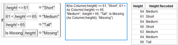
• Select Formula from the Column Properties menu in a New Column dialog and click the Edit Formula button that appears.
• Right-click (Windows) or Control-click (Macintosh) in the heading of a column or on the column in the Columns panel and select Formula from the context menu that appears. This opens the Formula Editor window without first opening the Column Info dialog.
The Formula Editor window is divided into two areas: the control panel, consisting of the column list and functions browser, and the formula display, an area for editing formulas. Figure 4.1 shows the parts of the Formula Editor, with a formula for the conversion from temperature in degrees Fahrenheit to Celsius. The Formula Editor control panel is composed of buttons (OK, Apply, Help), selection lists for variables and functions, and a keypad. The formula display is an editing area you use to construct and modify formulas.
Figure 4.1 The Formula Editor Window

The sections that follow show you a simple example, define Formula Editor terminology, and give the details for using the control panel and the formula display.
The Formula Editor and the JMP Scripting Language
Whenever you create a formula with the Formula Editor you are actually creating a JMP script. To see the script, double-click the formula. The script for the temperature conversion formula above is shown here.
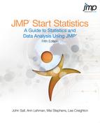
A more advanced but valuable example is recoding a continuous variable into discrete bins. For example, suppose you have a column of numeric Height values that you want to recode into three levels called “Short”, “Medium” and “Tall”. You could create a new column with the formula shown to the left in Figure 4.2. If you double-click on the formula, you’ll see the JSL statement in the middle. Columns with the original values and the recoded values are on the right in Figure 4.2.
Figure 4.2 Recode Formula and JSL
A Quick Example
The following example gives you a quick look at the basic features of the Formula Editor. Suppose you want to compute a standardized value. That is, for a numeric variable x, compute
where  is mean of x1, x2, x3,..., xi and
sx is the standard deviation of x1, x2, x3,..., xi
for each row in a data table.
It has a column called weight, and you want a new column that uses the above formula to generate standardized weight values.
The New Column dialog lets you set the new column’s characteristics.
The other default column characteristics define a numeric continuous variable and are correct for this example.
This opens the Formula Editor window shown previously in Figure 4.1.
Figure 4.3 The New Column Dialog
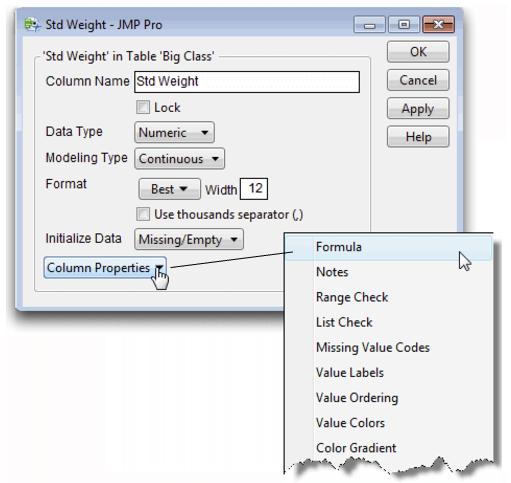
Next, enter the formula that standardizes the weight values by following the steps in Figure 4.4.
Figure 4.4 Entering a Formula
You have now entered your first formula.
The new column fills with values. If you change any of the weight values, the calculated Std Weight values automatically recompute.
If you make a mistake entering a formula, choose Undo from the Edit menu. There are other editing commands to help you modify formulas, including Cut, Copy, and Paste. The Delete key removes selected expressions. If you need to rearrange terms or expressions, you can select and drag to move formula pieces.
This example may be all you need to proceed. However, the rest of the chapter covers details about the Formula Editor, and gives a variety of other examples. Complete documentation of the Formula Editor is found in the Using JMP book, found in Help > Books.
Formula Editor: Pieces and Parts
This section begins with Formula Editor terminology. The Formula Editor has distinct areas, so we also describe its geography in more depth. Lastly, this section gives a brief description of all the function categories. Later sections give examples of specific functions.
Terminology
The following list is a glossary of terminology used when discussing the Formula Editor:
• A function is a mathematical or logical operation that performs a specific action on one or more arguments. Functions include most items in the function list and all keypad operators.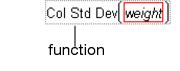
• An expression is a formula (or any part of it) that can be highlighted as a single unit, including terms, empty terms, and functions grouped with their arguments.
• A term is an indivisible part of an expression. Constants and variables are terms.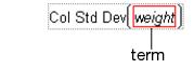
• An argument is a constant, a column, or expression (including mathematical operands) that is operated on by the function. Note: When you see a carat in the formula, click the carat (insert) button in the key pad to add a new argument.

• An empty term is a placeholder for an expression, represented by a small empty box.
• A missing value in a table cell shows as a missing value mark (a large dot) for numeric data, or a null character string for character data.
Figure 4.5 Missing Values

The Formula Editor Control Panel
The top part of the Formula Editor is called the control panel. It is composed of buttons and selection lists as illustrated in Figure 4.6.
Figure 4.6 The Formula Editor Control Panel
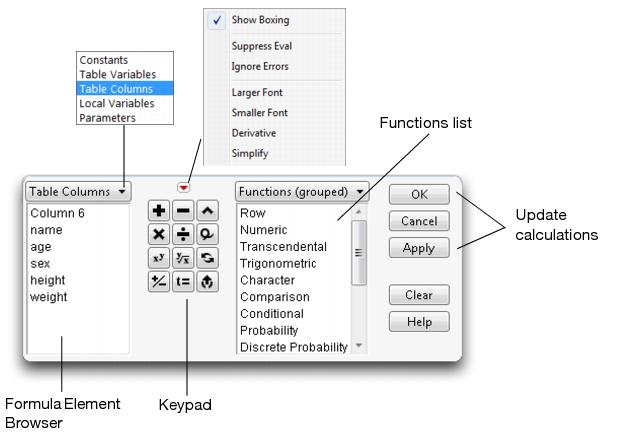
Some of the Formula Editor features, like those in the keypad, behave like those on a hand-held calculator. Other features are unique to the JMP Formula Editor. The following descriptions refer to Figure 4.6.
The Formula Element browser displays selection lists of table columns, constants, variables or parameters. By default, the list of table columns is visible. You can change the kind of elements listed by choosing from the menu at the top of the formula element browser. To choose a formula element, select an expression in the formula editing area, then select an element in the function list (see Figure 4.6).
The keypad is a set of buttons used to build formulas. Some of the buttons, such as the arithmetic operators, are familiar. Others have special functions, described in the next section.
The Function list groups collections of functions and features organized by topic. To use a function in a formula, select an expression in the editing area and click any item in one of the function groups. You can also see a list of ungrouped functions in alphabetical order by selecting Functions (All) from the menu above the function list.
The data table columns automatically fill with calculated values whenever you change a formula and then close the Formula Editor window or make it inactive. Use the Apply button to calculate a column’s values if you want the Formula Editor window to remain open.
The menu above the keypad (shown in Figure 4.6) has these commands:
• Show Boxing outlines terms within the formula. Boxing is important when you want to select and modify a specific portion of a formula, or need to determine the order of evaluation that takes place.
• Suppress Eval suppresses formula evaluation unless you specifically click Apply on the Formula Editor. This is a useful development mode when building complex formulas. You can turn off evaluation and build sections of a formula, then evaluate only to test the formula. In particular, you can close the Formula Editor and reopen it at a later time to continue building a formula without evaluating the formula.
• Ignore Errors suppresses error messages while a formula is under development. This is useful in situations where you want to see an evaluation for some rows and don’t want to see an error message for every row where the formula evaluation finds problems. If you don’t select Ignore Errors, an error message dialog appears when there is an error and asks if you want to ignore further errors. This has the same effect as the Ignore Errors menu selection.
• Larger Font increases the font size of the displayed formula.
• Smaller Font decreases the font size of the displayed formula.
• Derivative takes the first derivative of the entire formula. To use this command, first select a variable for the derivative to be taken with respect to. Then, select the Derivative command from the menu. This procedure is illustrated in Figure 4.7.
Figure 4.7 Derivatives in the Formula Editor

• Simplify algebraically simplifies the formula. For example, the Simplify command turns 2*x + 3*x into 5*x.
The Keypad Functions
The keypad is composed of common operators (referred to as functions here). Enter a keypad function by selecting an expression in the formula display and clicking on the appropriate keypad buttons.
Arithmetic keys
The four arithmetic functions work as they do on a pocket calculator.
Insert and Delete keys
The Insert button inserts a new empty formula clause or function argument. To insert a clause into a formula, first select the existing clause or argument you want the new element to follow. When you click the Insert button, the new clause appears and is selected. (Hint: You can also insert a new clause or argument by using the Insert keyboard shortcut: a comma.) The Delete button empties the selected box, or, if it is already empty, removes it as an argument.
Raise to a Power
The general exponential function raises a given value to a specified power. It has an exponent of two by default. Select the exponent and double-click on it to change its value.
Root
The root function calculates the specified root of the radicand. It has an implied index of 2, which is not displayed. To change the index to another value, highlight the argument of the root (the part outside the radical) and double-click to change its value.
Switch Terms
The switch terms keypad function looks at the operator that is central to the selected expression and switches the expressions on either side of that operator. For example, switching a + b results in b + a.
Unary Sign Function
The unary sign function inverts the sign of its argument. Apply the function to a selected variable expression or use it to enter negative constants.
Local Variable Assignment Key
This keypad function creates a local variable and assigns it the value of the selected expression. Its value can be as simple as an empty term, or as complicated as a complex formula.
Peel Expression
To use this function, begin by selecting any expression. When you click the Peel Expression button, the selected expression is deleted, leaving a selected empty term in its place. This process repeats each time the key is clicked. In this way, you can delete a formula term by term, in the precedence order of the formula, beginning with the first term you select. See the section Tips on Editing a Formula for a demonstration of peeling expressions.
The Formula Display Area
The formula display area or editing area (see Figure 4.1) is where you build and view a formula. To compose a formula, select expressions in the formula display area and apply functions and terms from the formula control panel.
Functions always operate upon selected expressions, terms always replace selected expressions, and arguments are always grouped with functions. To find which expressions serve as a function’s arguments, select that function in the formula. When the Show Boxing option is in effect, the boxed groupings also show how the order of precedence rules apply and show which arguments are deleted if you delete a function.
Function Definitions
The function categories are briefly described in the following list. They are presented in the order you find them in the function list. Examples of some commonly used functions are included later in this chapter.
• Row includes miscellaneous functions such as Lag, Dif, Subscript, Row (the current row number), and N Row (the total number of rows).
• Numeric includes the following functions: Abs (absolute value), Modulo, Ceiling, Floor and Round.
• Transcendental supports logarithmic functions for any base, functions for combinatorical calculations, the beta function, and several gamma functions.
• Trigonometric provides the standard trigonometric and hyperbolic functions such as sine, cosine, tangent, inverse functions, and their hyperbolic equivalents.
• Character has functions that operate on character arguments for, among other things, trimming, finding the length of a string, and changing numbers to characters or characters to numbers.
• Comparison includes the standard logical comparisons such as less than, less than or equal to, not equal to, and so forth.
• Conditional includes the logical functions Not, And, and Or. It also includes programming-like functions such as If, Match, and Choose.
• Probability provides functions that compute probabilities and quantiles for the Beta, chi-square, F, gamma, Normal, Student’s t, and a variety of other continuous distributions.
• Discrete Probability provides functions for the Poisson, Binomial, Hypergeometric and other discrete probability distributions.
• Statistical provides functions that calculate standard statistical quantities such as the mean or standard deviation, both down columns or across rows.
• Random is a collection of functions that generate random numbers from a variety of distributions.
• Date Time are functions that require arguments with the date data type, which is interpreted as the number of seconds since January 1, 1904. You assign Date as the Data Type in a New Column or Column Info dialog. Date functions return values such as day, week, or month of the year, compute dates, and can find date intervals.
• Row State includes functions that assign or detect special row characteristics called row states. Row states include color, marker, label, hidden (in plots), excluded (from analyses), selected or not selected and more.
• Assignment functions work in place. That is, the result returned by the operation (on the right of the operator) is stored in the argument on the left of the operator and replaces its current value. They are named constants that you create and can use in any formula.
• Parametric Model provides a shortcut to create three parametric models (linear, interactions and quadratic) that are linear functions of set of window-selected columns.
• Finance includes functions used in business and financial settings, such as principal payments, interest rate, rate or return, and net present value.
Row Function Examples
To do the next examples, create an empty data table and add some rows and columns to the table.
The first category in the function list is called Row. Click Row to see the menu of functions shown below.Because the Row functions are especially critical to building JMP formulas and have a variety of syntax, these functions are described in more detail than others.
Sequence
produces a sequence of numbers in a column using the start value, ending value, and increments that are specified as arguments.
Count
creates a list of stepped values beginning with the from value and ending with the to value. The number of steps specifies the number of values in the list.
Lag(column,n)
returns the value of the specified column in the row defined by the current row less the second argument. That is, it returns the value of column n rows back. The default lag is one, which you can change to any number. The value returned for any lag that identifies a row number less than one is missing. Note that Lag(X,n) gives the same result as the subscripted notation, XRow()–n. But Lag is more general, supporting entire expressions as well as simple column names.
Row()
is the current row number when an expression is evaluated for that row. You can incorporate this function in any expression, including those used as column name subscripts (discussed in the next section).
Dif(column,n)
returns the difference between the value of the column in the current row and the value n rows previous.
N Row ()
is the total number of rows in the data table.
Subscript
enables you to use a column’s value from a row other than the current row. Highlight a column name in the formula display and click Subscript to display a placeholder for the subscript. The placeholder can be changed to any numeric expression. Subscripts that evaluate to nonexistent row numbers produce missing values or, possibly, error messages. A column name without a subscript refers to the current row. To remove a subscript from a column, select the subscript and delete it. Then delete the empty box that remains. The formula
CountRow( )–CountRow( )–1
uses the subscript of Row()–1 to calculate the difference of two successive rows in a column named Count. Note that the subscript of Row() alone is not essential, since it refers to the current row, which is the default behavior.
The following formula calculates values for a a column called Fib, which, after the formula is evaluated, contains the terms of the Fibonacci series (each value is the sum of the two preceding values in the calculated column).

It shows the use of subscripts to do recursive calculations. A recursive formula includes the name of the calculated column, subscripted such that it references previously evaluated rows.
Using a Subscript
Use a subscript to refer to a specific row of the subscripted column. A simple use for subscripts is to create a lag variable similar to the Lag function. Follow these steps to create a lag variable:
Build the lag formula with these steps for the Lag column.
You should now see the lag formula: 
Don’t be alarmed by the invalid row number error message. Simply click Continue to continue with the formula evaluation. The Lag function refers to the row previous to the current row; at row 1, this results in referring to the non-existent row 0, which produces a missing value in the data table.
Note that the values in RowID and Lag are functions of individual rows, but the constant value in the Total Rows column is a function of the data table.
Figure 4.8 Formula Example
Conditional Expressions and Comparison Operators
The Conditional function category has many familiar programming functions This section shows examples of conditionals used with comparison operators..
The most basic and general conditional function is the If function. Its arguments are called If, Then, and Else clauses.
When you highlight an expression and click If, the Formula Editor creates a new conditional expression. It has one If argument (a conditional expression denoted expr), one argument, and a corresponding else and else clause. A conditional is usually an expression, like a < b.
However, any expression that evaluates as a numeric value can be used as a conditional expression. Expressions that evaluate as zero or missing are false. All other numeric expressions are true. An initial If expression looks like the one shown here.
If you need more than one then statement, click the insert button (the carat) on the keypad (or type a comma, its keyboard shortcut) to add a new argument. To remove unwanted arguments, use the delete icon on the keypad or hit the Delete key on your keyboard.
Using the If, Row, and Subscript functions
The formula for the Fibonacci sequence shown earlier uses the following functions: If, Row, Fib, and Subscript. As an exercise, create a Fibonacci sequence as follows:
Figure 4.9 Entering the Fibonacci Sequence Formula

Figure 14.9 (continued)

When you close the Formula Editor by clicking OK, the formula you entered generates the values shown in the first column in Figure 4.10.
Figure 4.10 Results of the Formula Example

The Fibonacci sequence has interesting and easy-to-understand properties that are discussed in many number theory textbooks.

Using the Match Function
A common use for conditional functions is to re-code variables. Often, a numeric coding variable represents a descriptive character value. The following example uses the Match function for re-coding (the If function could also be used).
Note: Value labels can also be used to add a descriptive label to a column of numeric variables. Details on value labels and their use are in the Using JMP book found in Help > Books.
When you select Match from the Conditional menu, the Formula Editor shows a single Match condition with an empty expression and an empty then term. You add and delete clauses in a Match conditional the same way as in the If conditional described previously: select a then clause and click the add or delete button. The Match conditional compares an expression to a list of clauses and returns the value of the result expression for the first matching argument encountered. With Match, you provide the matching expression only once and then give a match for each argument.
As an example, open the Hot dogs.jmp data table. Suppose you want to create a value to re-code the protein/fat ratio into categories “Very Lean,” “Lean,” “Average,” and so on (see the formula below).

Note: Match evaluates faster and uses less memory than an equivalent If.
By the way, a newer feature in JMP, Columns > Recode, gives another way to easily create a new column with coded values. For example, using the previously created column, Protein/Fat 2, let’s create an additional column with only three categories.

Figure 4.11 Recoding with Columns > Recode

Summarize Down Columns or Across Rows
The Formula Editor evaluates statistical functions differently from other functions. Most functions evaluate data only for the current row. However, all Statistical functions require a set of values upon which to operate. Some Statistical functions compute statistics for the set of values in a column, and other functions compute statistics for the set of arguments you provide.
The functions with names prefaced by “Col” (Col Mean, Col Sum, and so on) always evaluate for all of the rows in a column. Thus, used alone as a column formula, these functions produce the same value for each row. These functions accept only a single argument, which can be a column name, or an expression involving any combination of column names, constants, or other functions.
The other statistical functions (Mean, Std Dev, and so on) accept multiple arguments that can be variables, constants, and expressions.
The Sum and Product functions evaluate over an explicitly specified range of values.
The Quantile Function
The Col Quantile function computes a quantile for a column of n nonmissing values. The Col Quantile function’s quantile argument (call it p) represents the quantile percentage divided by 100.
The following examples are quantile formulas for a column named age:
Col Quantile (age, 1) finds the maximum age.
Col Quantile (age, 0.75) calculates the upper quartile age.
Col Quantile (age, 0.5) calculates the median age.
Col Quantile (age, 0.25) calculates the lower quartile age.
Col Quantile (age, 0.0) calculates the minimum age.
The pth quantile value is calculated using the formula I = p(N + 1) where p is the quantile and N is the total number of nonmissing values. If I is an integer, then the quantile value is yp = yi. If I is not an integer, then the value is interpolated by assigning the integer part of the result to i, and the fractional part to f, and by applying the formula
Using the Summation Function
The Summation (Σ) function uses the summation notation shown to the left. To calculate a sum, select Summation from the Statistical function menu and create its argument. The Summation function repeatedly evaluates the expression for the index you apply to the body of the function from the lower summation limit to the upper summation limit, and then adds the nonmissing results together to determine the final result. You can replace the index i, the index constant 1, and the upper limit, NRow(), with any expressions appropriate for your formula. Use the Subscript function in the Row function category to create a subscript for the body of the summation.
For example, the summation shown here computes the total of all revenue values for row 1 through the current row number, filling the calculated column with the cumulative totals of the revenue column.
Let’s see how to compute a moving average using the summation function.
Note that there is a column in the table called Moving Average—use this column and its formula as a reference.
When you specify Formula as a new column property, the new column appears in the table with missing values, and the Formula Editor window opens. You should see a table like the one shown in Figure 4.12.
Figure 4.12 Example Table for Building a Moving Average

A moving average is the average of a fixed number of consecutive values in a column, updated for each row. The following example shows you how to compute a 10-day moving average for Close, the closing price of a high tech stock. This means that for each row the Formula Editor computes the sum of the current Close value with the nine preceding values, then divides that sum by 10.


Now tailor the summation indices to sum just the 10 values you want:

An empty subscript now appears with the summation body.


To finish the moving average formula, you want to divide the sum by 10, but not start the averaging process until you actually have 10 values to work with.

 When you click Apply or close the Formula Editor, the Moving Average 2 column fills with values.
 Now generate a plot to see the result of your efforts.
You then see the plot in Figure 4.13, which compares closing stock values with their ten-day moving average.
Figure 4.13 Plot of Close and Its Moving Average over Date
Random Number Functions
Random number functions generate real numbers by essentially ‘rolling the dice’ within the constraints of the specified distribution. You can use the random number functions with a default ‘seed’ that provides a pseudo-random starting point for the random series, or use the Random Reset function and give a specific starting seed. Figure 4.14 shows JMP’s extensive random number menu.
Figure 4.14 Random Functions Menu in Column Calculator

Each time you click Apply in the Formula Editor window, random number functions produce a new set of numbers. This section shows examples of three commonly used random functions, Uniform, Normal and Column Shuffle.
Note: Random numbers in JMP are calculated using the Mersenne-Twister technique, far more efficient than in older versions of JMP. However, if you want to use the older functions, the JMP Scripting Language provides RandomSeededNormal and RandomSeededUniform. Their seed is set using the Random Seed function.
The Uniform Distribution
The Uniform function generates random numbers uniformly distributed between 0 and 1. This means that any number between 0 and 1 is as likely to occur as any other. You can use the Uniform function to generate any set of numbers by modifying the function with the appropriate constants.
You can see simulated distributions using the Uniform function and the Distribution platform.
Follow the same steps as before, except modify the Uniform function to generate the integers from 1 to 10 as follows.
Note: JMP has a Random Integer(n) function that selects integers from a uniform distribution from 1 to n. It could be used here for the same effect. We’re using the Random Uniform function to illustrate how to manipulate a random number by multiplying and adding constants. You can see an example of the Random Integer function in Rolling Dice.
The next steps are the key to generating a uniform distribution of integers (as opposed to real numbers as in Column 1):
The final formula is
Floor(Random Uniform()*10+1)
You now have a table template for creating two uniform distributions. Add as many columns as you want.
The table fills with values.
You see two histograms similar to those shown in Figure 4.15. The histogram on the left represents simple uniform random numbers and the histogram on the right shows random integers from 1 to 10.
Figure 4.15 Example of Two Uniform Distribution Simulations
The Normal Distribution
Random Normal generates random numbers that approximate a Normal distribution with a mean of 0 and variance of 1. The Normal distribution is bell-shaped and symmetrical. You can modify the Random Normal function with arguments that specify a Normal distribution with a different mean and standard deviation.
As an exercise, follow the same instructions described previously for the Uniform random number function.
The Random Normal function takes two optional arguments. The first specifies the mean of the distribution; the second specifies the standard deviation of the distribution.
The modified Normal formula is
Random Normal(30, 5)
Figure 4.16 shows the Distribution platform results for these Normal simulations.
Figure 4.16 Illustration of Normal Distributions

The Col Shuffle Command
Col Shuffle selects a row number at random from the current data table. Each row number is selected only once. When Col Shuffle is used as a subscript, it returns a value selected at random from the column that serves as its argument.
For example, to identify a 50% random sample without replacement, use the following formula:
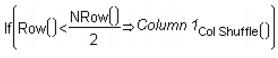
This formula chooses half the values (n/2) from Column 1 and assigns them to the first half of the rows in the computed column. The remaining rows of the computed column remain missing.
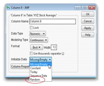
Initialize Data Options
When you add a new column to a data table, the Initialize Data menu in the Column Info window (shown in Figure 4.17) allows you to specify the type of initial data values for the new column. The default is Missing/Empty. The Random option provides populates the column with random data without accessing the Formula Editor or storing a formula in the column.
Figure 4.17 Initialize Data Options
Local Variables and Table Variables
Local variables let you define temporary numeric variables to use in expressions. Local variables exist only for the column in which they are defined.
To create a new local variable, use the button on the formula editor keypad. This button adds a temporary local variable to the formula editing area, which appears as a command ending in a semicolon. Alternatively, you can select Local Variables from the Formula Elements menu, select New Local, and complete the dialog that appears.
By default, local variables have the names t1, t2, and so on, and initially have missing values. Local variables appear in a formula as bold italic terms.
Optionally, you can create a local variable, change its name and assign a starting value in the Local Variable dialog. To use the Local Variable dialog, select Local Variables from the Formula Elements popup menu, then select New Local and complete the dialog, as illustrated here.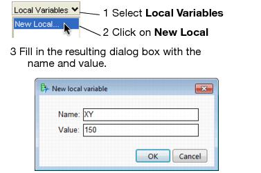
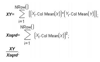
As an example, suppose you have variables x and y and you want to compute the slope in a simple linear regression of y on x using the standard formula shown here.
One way to do this is to create two local variables, called XY and Xsqrd, as described in the numerator and denominator in the equation above. Then assign them to the numerator and the denominator calculations of the slope formula. The slope computation is simplified to XY divided by Xsqrd.
The Local Variables command in the Formula Editor menu lists all the local variables that have been created.
Table variables are available to the entire table. Table variable names are displayed in the Tables panel at the left of the data grid. The Formula Editor can refer to a table variable in a formula.
Many of the sample data files have a table variable called Notes. The Table Variables command in the Formula Elements menu lists all the Table variables that exist for a table. You can create additional Table variables with the New Table Variable command in the Tables panel of the data table, or edit the values of existing table variables.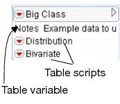
Some Nice Examples Involving Dates
Working with dates can present a challenge. Below are some frequently encountered example formulas involving dates.
Calculating Elapsed Time
Columns storing dates should be formatted as dates in the Column Info dialog. JMP dates are stored as the number of seconds since Jan 1, 1904. To create the elapsed time in days (or minutes, hours,...) between two date-formatted columns, requires the appropriate conversion formula. The formula shown here converts the elapsed time in seconds between Date 1 and Date 2 to days.
Age in Days
A variation of the elapsed time problem is calculating age (in days, minutes,...). This formula calculates the age in days between a date-formatted column and today using the Floor and Today functions.
Fixing Unformatted Dates
If dates have been entered into JMP in a character format, they can be converted to numeric date formats using a few key functions: Num, Word and Substr (all under the Characters function group).
The formula shown here parses the character string and converts the dates in the Date column to a numeric format. Note that the formula returns values in “raw” format (number of seconds since Jan 1, 1904). Change the date format in the Column Info window to display as a date.
Tips on Building Formulas
Examining Expression Values
Once JMP has evaluated a formula, you can select an expression to see its value. This is true for both parameters and expressions that evaluate to a constant value. To do this, select the expression you want to know about and right-click (PC) or control-click (Mac) on it. This displays a popup menu as shown here. When you select Evaluate, the current value of the selected expression shows until you move the cursor.
Cutting, Dragging, and Pasting Formulas
You can cut or copy a formula or an expression, and paste it into another formula display. Or you can drag any selected part of a formula to another location within the same formula. When you place the arrow cursor inside an expression and click, the expression is highlighted. When the cursor is over a selected area, it changes to a hand cursor, indicating that you can drag the highlighted formula under the cursor. As you drag across the formula, destination expressions are highlighted. When you release the drag, the selected expression is copied to the new location where it replaces the existing expression.
When you copy (or drag) an expression from one data table to another, JMP expects to find matching column names. If a formula column name does not appear in the destination table, an error alerts you when the formula attempts to evaluate.
Selecting Expressions
You can click on any single term in an expression to select it for editing. You can use the keyboard arrow keys to select expressions for editing or to view the grouping of terms within a formula when parentheses are not present or the boxing option is not in effect.
Once an operand is selected, the left and right arrow keys move the selection across other associative operands within the expression. The left arrow highlights the next formula element to the left of the currently highlighted term, or extends the selection to include an additional term that is part of a group.
Tip: Turn the boxing option on to see how the elements and terms are grouped in a formula you create. It is often easier to leave the boxing option on while creating a formula.
The up arrow on your keyboard extends the current selection by adding the next operand and operator of the formula term to the selection. The down arrow reduces the current selection by removing an operand and operator from the selection.
Tips on Editing a Formula
If you need to change a formula, highlight the column and select Formula from the Cols menu. Alternatively, right-click at the top of the column or on the column name in the Columns panel and select Formula from the context menu that appears.
Deleting a function also deletes its arguments. Deleting a required argument or empty term from a function sometimes deletes the function as well. You can save complicated expressions that serve as arguments and paste them where needed by using the Copy command to copy the arguments to the clipboard.
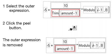
Another useful editing technique is to peel a function from its argument as shown in Figure 4.18. To peel a function from a single argument, first click to select the function. Then, choose the peel button from the keypad, as shown in Figure 4.18.
After you complete formula changes, the new values fill the column automatically when you click Apply or close the Formula Editor window.
Once you have created a formula, you can change values in columns that are referenced by your formula. JMP automatically recalculates all affected values in the formula’s column.
Figure 4.18 Peeling Expressions or Arguments
Exercises
1. The file Pendulum.jmp contains the results of an experiment in a physics class comparing the length of a pendulum to its period (the time it takes the pendulum to make a complete swing). Calculations were made for a range of pendulums from short (2 cm) to long (20 m). We will use the calculator to determine a model to predict the period of a pendulum from its length.
(a) Produce a scatterplot of the data by selecting Analyze > Fit Y By X and selecting Period as the Y variable and Length as the X variable.
(b) Create a new column named Transformed Period that contains a formula to take the square root of the Period column. Produce a scatterplot of Transformed Period vs. Length. Is this the graph of a linear function?
(c) Try other transformations (for example, natural log of Period, reciprocal of Period, or square of Period) until the scatterplot looks linear.
(d) Find the line of best fit for the linear transformed data by selecting Fit Line from the popup menu beside the title of the scatterplot.
(e) This line is not the fit of the original data, but of the transformed data. Substitute a term representing the transformation you did to linearize the data (for example, if the square root transformation made the data linear, substitute  into the regression equation) and solve the equation for Period.
A Physics textbook reveals the relationship between period and length to be
(f) Create a new column to use this formula to calculate the theoretical values. Next, construct another column to calculate the difference between the observed values of the students and the theoretical values.
(g) Examine a histogram of these differences. Does it appear that there was a trend in the observations of the students?
2. Is there a correlation among the mean, minimum, maximum, and standard deviation of a set of data? To investigate, create a new data table in JMP with these characteristics:
(a) Create ten columns of data named Data 1 through Data 10, each with the formula Random Uniform(). Add 500 rows to this data table.
(b) Create four columns to hold the four summary statistics of interest, one column each for the mean, minimum, maximum, and standard deviation. Create a formula in each column to calculate the appropriate statistic of the ten data rows.
(c) Select the Multivariate platform in the Analyze > Multivariate Methods menu and include the four summary statistics as the Y’s in the resulting dialog box. Pressing OK should produce 16 scatterplots. Which statistics seem to show a correlation?
(d) As an extension, select two of the statistics that seem to show a correlation. Produce a single scatterplot of these two statistics using the Fit Y By X platform in the Analyze menu. From the red triangle menu beside the title of the plot, select Nonpar Density. Then choose Save Density Grid from the menu beside the density legend.
(e) Finally, select Graph > Scatterplot 3D and include the first three columns of the saved density grid. You should now see a 3D scatterplot of the correlation, with a peak where the data points overlapped each other. Use the hand tool to move the plot around.
3. Make a data table consisting of 20 rows and a single column that holds the Fibonacci sequence (whose formula is shown on ). Label this column Fib.
(a) Add a new column called Ratio, and give it the following formula to take the ratio of adjacent rows. Note: This will produce an error alert when evaluated for the first row. Click OK on the alert dialog to resolve this issue.
What value does this ratio converge to?
(b) A more generalized Fibonacci sequence uses values aside from 1 as the first two elements. A Lucas sequence uses the same recursive rule as the Fibonacci, but uses different starting values. Create a column to hold a Lucas sequence beginning with 2 and 5 called Lucas with the formula

(c) Create a column to calculate the ratio of two successive terms of the Lucas sequence in part (b). Is it the same as the number in part (a)?
(d) Create a Lucas sequence starting with the values 1, 2. Calculate the ratio of successive terms and compare it to the answer in part (c).
(e) There are innumerable other properties of the Fibonacci sequence. For example, add a column that contains the following formula, and comment on the result.
..................Content has been hidden....................
You can't read the all page of ebook, please click here login for view all page.