Chapter 16: Summarizing Your Data

16.1  Introduction

16.2  PROC MEANS—Starting from the Beginning

16.3  Adding a BY Statement to PROC MEANS

16.4  Using a CLASS Statement with PROC MEANS

16.5  Applying a Format to a CLASS Variable

16.6  Deciding between a BY Statement and a CLASS Statement

16.7  Creating Summary Data Sets Using PROC MEANS

16.8  Outputting Other Descriptive Statistics with PROC MEANS

16.9  Asking SAS to Name the Variables in the Output Data Set

16.10  Outputting a Summary Data Set: Including a BY Statement

16.11  Outputting a Summary Data Set: Using a CLASS Statement

16.12  Using Two CLASS Variables with PROC MEANS

16.13  Selecting Different Statistics for Each Variable

16.14  Printing all Possible Combinations of Your Class Variables

16.15  Problems

 

You may have thought of PROC MEANS (or PROC SUMMARY) primarily as a way to generate summary reports, reporting the sums and means of your numeric variables. However, these procedures are much more versatile and can be used to create summary data sets that can then be analyzed with more DATA or PROC steps.

All the examples in this chapter use PROC MEANS rather than PROC SUMMARY, even when all you want is an output data set. The reason for this is that using PROC MEANS with a NOPRINT option is identical to using PROC SUMMARY when you are creating an output data set.

You can begin by running PROC MEANS with all the defaults, using the permanent SAS data set Blood.

 

Here it is:

Program 16.1: PROC MEANS with All the Defaults

Here is the resulting output:

Figure 16.1: Output from Program 16.1

By default, PROC MEANS produces statistics on all the numeric variables in the input SAS data set. Looking at the output, you see the default statistics produced are N (number of nonmissing values), Mean (average), Std Dev (standard deviation), Minimum, and Maximum. The next step is to gain some control over this process.

You can control which variables to include in the report by supplying a VAR statement. Statistics are chosen by selecting options in the PROC MEANS statement. Here is a partial list of some of the more commonly used options.

PROC MEANS Option	Statistic Produced
N	Number of nonmissing values
NMISS	Number of missing values
MEAN CLM	Mean or Average Confidence Limit for the Mean
SUM	Sum of the values
MIN	Minimum (nonmissing) value
MAX	Maximum value
MEDIAN	Median value
STD	Standard deviation
VAR	Variance
CLM	95% confidence interval for the mean
Q1	Value of the first quartile (25th percentile)
Q3	Value of the third quartile (75th percentile)
QRANGE	Interquartile range (equal to Q3–Q1)

Besides these statistics, the option MAXDEC=value is especially useful. This value controls the number of places to the right of the decimal point that are printed in the output.

Let’s use some of these options to customize the output. You will compute the number of missing and nonmissing values, the mean, median, minimum, and maximum for the variables RBC (red blood cells) and WBC (white blood cells) in the Blood data set. Finally, you will report all statistics to the nearest 10th. Here is the program:

Program 16.2: Adding a VAR Statement and Requesting Specific Statistics with PROC MEANS

The output follows:

Figure 16.2: Output from Program 16.2

You now have only the statistics you requested on the variables listed in the VAR list. Notice also that all the statistics are reported to one decimal place, due to the MAXDEC=1 option. (Unfortunately, the number of decimal places you choose is applied to all variables. If you need more control over the number of printed decimal places for each variable, you can use PROC TABULATE.) Values for N and NMISS are always integers.

If you want to see descriptive statistics for each level of another variable, you can include a BY statement, listing one or more BY variables. Remember that you have to sort your data set first by the same variable or variables you list in the BY statement. Here are the same statistics displayed by Figure 16.2, broken down by gender:

Program 16.3: Adding a BY Statement to PROC MEANS

You now have your descriptive statistics for males and females separately, as shown next:

Figure 16.3: Output from Program 16.3

PROC MEANS lets you use a CLASS statement in place of a BY statement. The CLASS statement performs a similar function to the BY statement, with some significant differences. If you are using PROC MEANS to print a report and are not creating a summary output data set, the differences in the printed output between a BY and CLASS statement are basically cosmetic. The main difference, from a programmer’s perspective, is that you do not have to sort your data set before using a CLASS statement. To demonstrate this, run Program 16.3 again, substituting the CLASS statement for the BY statement, as follows:

Program 16.4: Using a CLASS Statement with PROC MEANS

Notice that you are using the permanent SAS data set (that may not be sorted) instead of the temporary sorted data set used in Program 16.3. There are some minor differences in the appearance of the printed output, as shown here:

Figure 16.4: Output from Program 16.4

One very nice feature of using a CLASS statement (besides not having to sort your data) is that SAS uses formatted values of the CLASS variable(s). You can use this to your advantage by adding a FORMAT statement to the procedure and changing how the CLASS variable groups your data, all without having to modify your original data set.

Suppose you want to see some basic statistics (mean and median) for the two blood count variables (RBC and WBC), broken down by subjects with cholesterol levels below 200 versus subjects with cholesterol levels at or above 200. See how easy this is to do with a CLASS statement and a FORMAT statement:

Program 16.5: Demonstrating the Effect of a Formatted CLASS Variable

Do you see the tremendous power in this method? You can try different groupings of CLASS variables by supplying a new format. Here is the output:

Figure 16.5: Output from Program 16.5

Even though the variable Chol (Cholesterol) is a continuous value, the output displays statistics for the formatted values of the variable.

There are a number of considerations in deciding whether to use a BY or a CLASS statement when you want to use PROC MEANS to produce printed output (the differences are more important if you are using PROC MEANS to create summary output data sets).

First, if you have a very large data set that is not sorted, you may want to use a CLASS statement. However, if the data set is already in the correct sorted order, you can use either a CLASS or a BY statement. If you have a large number of CLASS variables and there are many distinct values for each of these variables, you may need considerable computer memory to run the procedure. If you have relatively small data sets, choose the statement that produces the style of printed output that you prefer.

You can use PROC MEANS (or SUMMARY) to create a new data set that contains summary information such as sums and means. This data set can then be used for further analysis. This first example shows how to compute two means and output them to a SAS data set.

Program 16.6: Creating a Summary Data Set Using PROC MEANS

An OUTPUT statement tells PROC MEANS that you want to create a summary SAS data set. The keyword OUT= is used to name the new data set. In this example, you are going to name your output data set My_Summary. Next, you can specify exactly what statistics you want in this data set. You can output most of the statistics listed earlier in this chapter. Following the keyword and an equal sign, you provide a list of the variable names that correspond to these values. In this program, the variable MeanRBC is the mean of all the RBC values, and MeanWBC is the mean of all the WBC values. You can name these variables anything you want—they are arbitrary. The order of the variables here corresponds to the order of the variables in the VAR list. It is convenient to name these variables in a way that helps you remember what they stand for. Shortly, you will see that SAS can name these variables for you in a very convenient way. Finally, if you want to create a SAS data set but do not want any printed output from PROC MEANS, use the NOPRINT option. As we mentioned earlier, if you choose to use PROC SUMMARY instead of PROC MEANS, you do not need a NOPRINT option—it is the default for that procedure.

Program 16.6 also includes a PROC PRINT statement so that you can see the contents of the output data set. Here is the listing of the summary data set My_Summary:

Figure 16.6: Output from Program 16.6

This data set has only one observation. It includes the two means plus two additional variables created by PROC MEANS. We will discuss these two variables later when we run the procedure with a CLASS statement.

When you are outputting only a single statistic (such as a mean in the previous example), you can omit the variable list following the keyword MEAN= if you want. If you do, SAS gives these summary variables the same names as the variables listed in the VAR statement. It is strongly recommended that you do not do this. It is easy to make a mistake when you have the same variable name in two data sets, with one representing individual values and the other representing a summary statistic.

As we mentioned earlier, you can output more than one statistic in your output data set. As an example, let’s output the mean, the number of nonmissing observations, the number of missing observations, and the median. Here is the program:

 

Program 16.7: Outputting More Than One Statistic with PROC MEANS

So, you get the idea. You can output as many statistics as you want and name them anything you want. A listing of this data set, using PROC PRINT, is shown here:

Figure 16.7: Listing of Data Set Many_Stats

The two variables M_RBC and M_WBC represent the means of RBC and WBC, respectively. The two variables Med_RBC and Med_WBC are the medians of the two variables. N_RBC and N_WBC represent the number of nonmissing values; Miss_RBC and Miss_WBC represent the number of missing values for these two variables. As a check, notice that N_RBC plus Miss_RBC equals 1,000, the total number of observations in data set Blood.

You can ask SAS to create variable names for any of the summary statistics produced by PROC MEANS. The OUTPUT option AUTONAME causes PROC MEANS to create variable names for the selected statistics by using the variable names in the VAR statement and adding an underscore character followed by the name of the statistic. The best way to see this is to look at a program and a listing of the output data set:

Program 16.8: Demonstrating the OUTPUT Option AUTONAME

Because AUTONAME is a statement option, it follows a slash in the OUTPUT statement. Take a look at a listing of this data set to see how SAS named these variables:

Figure 16.8: Listing of Data Set Many_Stats

The OUTPUT option AUTONAME is quite useful, and it creates consistent and easy-to-understand variable names. Be aware that the suffix used for standard deviation is StdDev and not the abbreviation Std that is commonly used. Also remember that SAS variable names cannot be longer than 32 characters—this includes the suffix that PROC MEANS adds. Although it is unlikely, if adding the suffix causes the variable name to exceed 32 characters, the original variable name will be truncated.

Although there are many uses for a summary data set containing summary statistics on an entire data set, there are times when you would like to output summary statistics for each level of one or more classification variables. For example, you might want to see n's and means of RBC and WBC broken down by gender. Remember that to use a BY statement, the data set must be sorted in the same order. Program 16.9 creates a summary data set containing the mean values of RBC and WBC for males and females.

Program 16.9: Adding a BY Statement to PROC MEANS

A listing of the output data set follows:

Figure 16.9: Listing of Data Set By_Gender

In this data set, _FREQ_ represents the number of observations for each value of gender (it doesn’t matter if there are missing values for RBC or WBC). For example, you see that there are 440 females in the data set and that the means for RBC and WBC are 5.49848 and 7112.43, respectively. The variables RBC_N and WBC_N represent the number of nonmissing values that were used to compute the two means.

As you saw earlier in this chapter, you can use a CLASS statement with PROC MEANS to obtain results similar to those obtained using a BY statement. The difference between the two becomes more apparent when you are creating output data sets. The program here is a repeat of Program 16.9, with a CLASS statement replacing the BY statement (and the PROC SORT omitted):

Program 16.10: Adding a CLASS Statement to PROC MEANS

The resulting data set is listed here:

Figure 16.10: Listing of Data Set With_Class

Notice that you now have three observations instead of just two. The first observation in this data set, with _TYPE_ equal to 0, is the mean for both males and females. Statisticians call this the grand mean. The other two observations with _TYPE_ equal to 1 represent the means for females and males. We will discuss the interpretation of the _TYPE_ variable in the next section, which demonstrates the use of more than one CLASS variable.

If you only want the means broken down by gender and do not want an observation with the grand mean in your output data set, use the NWAY option of PROC MEANS. Using this option makes the output data set using a CLASS statement identical (except for the value of _TYPE_) to an output data set using a BY statement. Program 16.11 demonstrates the effect of the NWAY option:

 

Program 16.11: Adding the NWAY Option to PROC MEANS

The resulting data set is shown below:

Figure 16.11: Listing of Data Set With_Class

Notice that the extra observation containing the grand mean is no longer present.

Things start to get more complicated when you have more than one CLASS variable. Suppose you want to compute the mean and the number of nonmissing values for RBC and WBC for each combination of AgeGroup and Gender. You place these two variables in the CLASS statement and create an output data set just as you did earlier with only one CLASS variable. Here are the PROC statements to create such an output data set:

Program 16.12: Using Two CLASS Variables with PROC MEANS

 

And here is a listing of the output data set:

Figure 16.12: Listing of Data Set Summary

Notice that things are getting more complicated. Even though there are only two levels of Gender and two levels of AgeGroup, there are nine observations in the output data set with four values of _TYPE_. The _TYPE_ = 0 observation is the same as you saw earlier—it represents the grand mean, the mean of all nonmissing values in the data set. To understand the other observations in this data set, you have to know either how to count in binary or how to use another PROC MEANS option—CHARTYPE. Let’s take the easy way out and rerun this program with the CHARTYPE procedure option as follows:

Program 16.13: Adding the CHARTYPE Procedure Option to PROC MEANS

 

A listing of the output now looks like this:

Figure 16.13: Listing of Data Set Summary (with CHARTYPE Procedure Option)

This may not look any simpler, but it is now easier to explain what the variable _TYPE_ represents. First of all, the option CHARTYPE (this stands for character type) causes the _TYPE_ variable to be a character string of 1’s and 0’s. If you are familiar with counting in binary, you will observe that the character strings under the _TYPE_ column represent the previous _TYPE_ values, except they are now in a binary representation. (It’s OK if this last sentence is meaningless to you—that’s why SAS created the CHARTYPE option in the first place.)

If you look at the CLASS statement, you see the two variables Gender and AgeGroup. If you imagine writing the left-most character of _TYPE_ under Gender and the other character of _TYPE_ under AgeGroup, there is a simple rule for interpreting the summary statistic for any value of _TYPE_. The following table displays the CLASS variables with the values of _TYPE_ written underneath (we will use the mean as an example):

 

	Gender	AgeGroup	Interpretation
_TYPE_	0	0	Mean for all Genders and all AgeGroups
	0	1	Mean for each level of AgeGroup
	1	0	Mean for each level of Gender
	1	1	Mean for each combination of Gender and AgeGroup

Here is the rule: if there is a 1 under the CLASS variable, the statistics in the output data set represent the statistics computed on each level of that variable. For example, if you are computing means, the mean with a value of _TYPE_ equal to 10 is a mean computed at each level of Gender (for all age groups). If you only want the statistics broken down by each level of the CLASS variables, you can use the NWAY option. This selects only the largest value of _TYPE_. (If you use the CHARTYPE option, NWAY selects the value of _TYPE_ containing all 1’s.)

You can use the _TYPE_ variable to select the appropriate breakdown. For example, you can use the _TYPE_ values in a WHERE statement in a PROC PRINT statement, like this:

Program 16.14: Using the _TYPE_ Variable to Select CLASS Variable Breakdowns

Figure 16.14: Output from Program 16.14

Because the values are broken down by Gender, AgeGroup has a missing value in each observation (it was left in the listing for demonstration purposes).

You can also use this summary data set to create separate data sets: one for the grand mean, one for means broken down by Gender, one broken down by AgeGroup, and one containing cell means. You can do this in one DATA step, like this:

Program 16.15: Using a DATA Step to Create Separate Summary Data Sets

Because you want a different selection of variables in each data set, you can use a KEEP= or DROP= data set option to make your selection. Because you want to drop _TYPE_ from every data set, it is easier to do this with a DROP statement in the DATA step. A RENAME statement renames _FREQ_ to Number. Again, this change applies to all four data sets.

_TYPE_ is a character variable because of the CHARTYPE option, and you can use it to route each observation to the proper output data set.

Below are listings of the four data sets produced by Program 16.15:

Figure 16.15: Listing of the Four Data Sets Produced by Program 16.15

 

There is an alternative way of selecting which variables and statistics you want in your summary data set, as shown in Program 16.16.

Program 16.16: Selecting Different Statistics for Each Variable Using PROC MEANS

We have added several new features to this program. Each statistic keyword is followed by a list of variables (placed in parentheses) for which you want to compute this statistic. For example, this program computes means for RBC and WBC, the number of nonmissing values for all three variables (RBC, WBC, and Chol), and the median of Chol. Although you can name the newly created statistic following the equal sign as before, this program uses the AUTONAME output option to name them.

Finally, you may wonder about the rather strange-looking DROP= data set option in the SUMMARY data set. This DROP= option uses the colon wildcard notation. All variables beginning with an underscore character will be dropped. In general, name: used in any location where you would place a variable list refers to all variables beginning with the letters name. You can think of the colon the same way you use an asterisk as a DOS wildcard (if anyone still remembers DOS).

A listing of the Summary data set follows:

Figure 16.16: Listing of Data Set Summary

As you saw in the examples in this chapter, PROC MEANS can do a lot more than print summary statistics—it can create summary data sets broken down by one or more CLASS variables. By using options such as CHARTYPE and AUTONAME, you can simplify your programs and let SAS name your summary variables for you.

A very useful PROC MEANS option called PRINTALLTYPES prints summaries of every combination of your class variables. To demonstrate this, take a look at Program 16.17:

Program 16.17: Demonstrating the PRINTALLTYPES PROC MEANS Option

Adding this single option to PROC MEANS results in the following:

Figure 16.17: Output from Program 16.17

This really useful option was not available when I wrote the last edition of this book. I'm happy to share it with you.

Solutions to odd-numbered problems are located at the back of this book. Solutions to all problems are available to professors. If you are a professor, visit the book’s companion website at support.sas.com/cody for information about how to obtain the solutions to all problems.

1.       Using the SAS data set College, compute the mean, median, minimum, and maximum and the number of both missing and nonmissing values for the variables ClassRank and GPA. Report the statistics to two decimal places.

Repeat Problem 1, except compute the desired statistics for each combination of Gender and SchoolSize. Do this twice, once using a BY statement, and once using a CLASS statement. Note: The data set College has permanent formats for Gender, SchoolSize, and Scholarship. Either make this format catalog available to SAS (see Chapter 5), run the PROC FORMAT statements that follow, or use the system option NOFMTERR (no format error) that allows you to access SAS data sets that have permanent user-defined formats without causing an error.

  proc format;

     value $Yesno  'Y','1' = 'Yes'

                   'N','0' = 'No'

                   ' '   = 'Not Given';

     value $Size   'S' = 'Small'

                   'M' = 'Medium'

                   'L' = 'Large'

                   ' ' = 'Missing';

     value $Gender 'F' = 'Female'

                   'M' = 'Male'

                   ' ' = 'Not Given';

  run;

2.       Using the SAS data set College, report the mean and median GPA and ClassRank broken down by school size (SchoolSize). Do this twice, once using a BY statement, and once using a CLASS statement.

3.       Repeat Problem 3 (CLASS statement only), except group small and medium school sizes together. Do this by writing a new format for SchoolSize (values are S, M, and L). Do not use any DATA steps.

4.       Using the SAS data set College, report the mean GPA for the following categories of ClassRank: 0–50 = bottom half, 51–74 = 3rd quartile, and 75 to 100 = top quarter. Do this by creating an appropriate format. Do not use a DATA step.

5.       Using the SAS data set College, create a summary data set (call it Class_Summary) containing the n, mean, and median of ClassRank and GPA for each value of SchoolSize. Use a CLASS statement and be sure that the summary data set only contains statistics for each level of SchoolSize. Use the AUTONAME option to name the variables in this data set.

6.       Using the SAS data set College, create four summary data sets containing the number of nonmissing and missing values and the mean, minimum, and maximum for ClassRank and GPA, broken down by Gender and SchoolSize. The first data set (Grand) should contain the statistics for all subjects, the second data set (ByGender) should contain the statistics broken down by Gender, the third data set (BySize) should contain the statistics broken down by SchoolSize, and the fourth data set (Cell) should contain the statistics broken down by Gender and SchoolSize. Do this by using PROC MEANS (with a CLASS statement) and one DATA step.

Hint: Use the CHARTYPE procedure option.

7.       Using the SAS data set SASHELP.Cars, compute the mean and standard deviation for Horsepower broken down by Make and Origin. Include the number of nonmissing and missing values in the output and print all statistics to one decimal place. Use the PRINTALLTYPES option to see all possible combinations of the CLASS variables.

Use PROC PRINT (without any DATA steps) to create a listing like the one here.

Note: The variables in the Hosp data set are Subject, AdmitDate (Admission Date), DischrDate (Discharge Date), and DOB (Date of Birth).

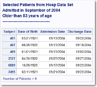
Hints: Variable labels replace variable names. The number of observations is printed at the bottom of the listing. There are four title lines (the last one being a dashed line).