Chapter 26: Introducing the Structured Query Language
26.3 Joining Two Tables (Merge)
26.4 Left, Right, and Full Joins
26.7 Demonstrating the ORDER Clause
26.8 An Example of Fuzzy Matching
PROC SQL (structured query language—usually pronounced sequel) offers an alternative to the DATA step for querying and combining SAS data sets. There are some tasks that PROC SQL can perform much better and easier than the DATA step. Other tasks may be easier or more efficient using a DATA step. You may also be more familiar with SQL versus the DATA step or vice versa. The best advice is to learn both and use the tool that works best for you in each situation.
This chapter only touches on the basics of PROC SQL. There are some excellent books published by SAS that you will probably want to own. Please check SAS Help Center at http://go.documentation.sas.com or books in the SAS Press series for more information on PROC SQL
Programmers familiar with SAS syntax may have some difficulty getting started with PROC SQL. For example, you use commas, not spaces, to separate variable and data set names in PROC SQL. You may also find yourself putting semicolons where they don’t belong. Let’s start out with some simple examples of querying a data set and creating a SAS data set by subsetting observations from a larger SAS data set.
Before we show you a program, a few words on terminology are in order. The following table lists SAS terms and the corresponding SQL terms:
|
SAS Term |
SQL Equivalent |
|
Data set |
Table |
|
Observation |
Row |
|
Variable |
Column |
For the first few examples, we will be working with a SAS data set called Health. Here is a listing:
Figure 26.1: Listing of Data Set Health

If you want to print a subset of this data set, selecting all subjects with heights over 65 inches, you could submit the following query:
Program 26.1: Demonstrating a Simple Query from a Single Data Set
title "Subjects from Health with Height > 65";
proc sql;
select Subj,
Height,
Weight
from Learn.Health
where Height gt 65;
quit;
This query starts with a SELECT keyword where you list the variables you want. Notice that the variables in this list are separated by commas (spaces do not work). The keyword FROM names the data set you want to read. Finally, a WHERE clause describes the particular subset you want.
SELECT, FROM, and WHERE form a single query, which you end with a single semicolon. In this example, you are not creating an output data set, so, by default, the result of this query is sent as a listing in the Output window (or whatever output location you have specified). Finally, the query ends with a QUIT statement. You do not need a RUN statement because PROC SQL executes as soon as a complete query has been specified. If you don’t include a QUIT statement, PROC SQL remains in memory for another query.
Here is the output that resulted from this program:
Figure 26.2: Output from Program 26.1

If you want to select all the variables from a data set, you can use an asterisk (*), like this:
Program 26.2: Using an Asterisk to Select all the Variables in a Data Set
proc sql;
select *
from Learn.Health
where Height gt 65;
quit;
If you want the result of the query to be stored in a SAS data set, include a CREATE TABLE statement, like this:
Program 26.3: Using PROC SQL to Create a SAS Data Set
proc sql;
create table Height65 as
select *
from Learn.Health
where Height gt 65;
quit;
Two tables, Health (used in the last example) and Demographic, are used to demonstrate various ways to perform joins using PROC SQL. Here are listings of these two tables:
Figure 26.3: Listing of Tables Health and Demographic

You can select variables from two tables by listing all the variables of interest in the SELECT clause and listing the two data sets in the FROM clause. If a variable has the same name in both data sets, you need a way to distinguish which data set to use. Here’s how it’s done:
Program 26.4: Joining Two Tables (Cartesian Product)
title "Demonstrating a Cartesian Product";
proc sql;
select Health.Subj,
Demographic.Subj,
Height,
Weight,
Name,
Gender
from Learn.Health,
Learn.Demographic;
quit;
Because the column Subj is in both tables, you prefix the variable name with the table name. You will see in a minute that you can simplify this a bit. The result from this query is called a Cartesian product and it represents all possible combinations of rows from the first table with rows from the second table. The listing shows two columns, both with the heading of Subj.
Here is a listing of the result:
Figure 26.4: Output from Program 26.4

If you use this same query to create a SAS data set, there will only be one variable called Subj. If you would like to keep both values of Subj from each data set, you can rename the columns, like this:
Program 26.5: Renaming the Two Subj Variables
title "Renaming the Two Subj Variables";
proc sql;
select Health.Subj as Health_Subj,
Demographic.Subj as Demog_Subj,
Height,
Weight,
Name,
Gender
from Learn.Health,
Learn.Demographic;
quit;
Running this query results in the following:
Figure 26.5: Partial Output from Program 26.5

Notice that the two subject columns are renamed.
A Cartesian product is especially useful when you want to perform matches between names in two tables that are similar (sometimes called a fuzzy merge). The number of rows in this table is the number of rows in the first table times the number of rows in the second table. In practice, you will want to add a WHERE clause to restrict which rows to select. In the program that follows, we add a WHERE clause to select only those rows where the subject number is the same in the two tables.
Besides adding a WHERE clause, the next program also shows how to distinguish between two columns both with a heading of Subj. Finally, this next program uses a simpler method of naming the two Subj variables in the SELECT clause. Here it is:
Program 26.6: Using Aliases to Simplify Naming Variables
title "Matching Subj Numbers from Both Tables";
proc sql;
select H.Subj as Subj_Health,
D.Subj as Subj_Demog,
Height,
Weight,
Name,
Gender
from Learn.Health as H,
Learn.Demographic as D
where H.Subj eq D.Subj;
quit;
First take a look at the FROM clause. To make it easier to name variables with the same name from different tables, you create aliases for each of the tables, H and D, in this program. You can use these aliases as a prefix in the SELECT clause (H.Subj and D.Subj). In this program, a WHERE clause was added, restricting the result to rows where the subject number is the same in both tables. Here is the result:
Figure 26.6: Matching Subj Numbers from Both Tables

Only subjects who are in both tables are listed here. In SQL terminology, this is called an inner join. It is equivalent to a merge in a DATA step where each of the two data sets contributes to the merge.
Just so this is clear, here is the same (well almost—in PROC SQL, you get two Subj variables) result using a DATA step:
Program 26.7: Performing an Inner Join Using a DATA Step
proc sort data=Learn.Health out=Health;
by Subj;
run;
proc sort data=Learn.Demographic out=Demographic;
by Subj;
run;
data Inner;
merge Health(in=in_Health)
Demographic(in=in_Demographic);
by Subj;
if in_Health and in_Demographic;
run;
title "Performing an Inner Join Using a DATA Step";
proc print data=Inner;
id Subj;
run;
Isn’t it nice that you don’t have to sort the data sets first when you use SQL? (Although PROC SQL does the sorts for you.) Below is a listing of the data set Inner:
Figure 26.7: Output from Program 26.7

This is identical to the PROC SQL table except for the fact that there is only one Subj variable.
An alternative to Program 26.6 is to separate the two table names with the term INNER JOIN, like this:
Program 26.8: Performing an Inner Join
title "Demonstrating an Inner Join (Merge)";
proc sql;
select H.Subj as Subj_Health,
D.Subj as Subj_Demog,
Height,
Weight,
Name,
Gender
from Learn.Health as H inner join
Learn.Demographic as D
on H.Subj eq D.Subj;
quit;
One of the rules of SQL is that when you use the keyword JOIN to join two tables, you use an ON clause instead of a WHERE clause. (You may further subset the result with a WHERE clause.)
If you write your inner join this way, it is easy to replace the term INNER JOIN with one of the following: LEFT JOIN, RIGHT JOIN, or FULL JOIN.
A left join includes all the rows from the first (left) table and those rows from the second table where there is a corresponding value in the first table. A right join includes all rows from the second (right) table and only matching rows from the first table. A full join includes all rows from both tables (equivalent to a merge in a DATA step). The following program demonstrates these three joins:
Program 26.9: Demonstrating a Left, Right, and Full Join
proc sql;
title "Left Join";
select H.Subj as Subj_Health,
D.Subj as Subj_Demog,
Height,
Gender
from Learn.Health as H left join
Learn.demographic as D
on H.Subj eq D.Subj;
title "Right Join";
select H.Subj as Subj_Health,
D.Subj as Subj_Demog,
Height,
Gender
from Learn.Health as H right join
Learn.demographic as D
on H.Subj eq D.Subj;
title "Full Join";
select H.Subj as Subj_Health,
D.Subj as Subj_Demog,
Height,
Gender
from Learn.health as H full join
Learn.demographic as D
on H.Subj eq D.Subj;
quit;
The results are as follows:
Figure 26.8: Output from Program 26.9

Inspection of this output should help make clear the distinctions among the different types of joins.
In a DATA step, you concatenate two data sets by naming them in a single SET statement. In PROC SQL, you use a UNION operator to concatenate selections from two tables. Unlike the DATA step, there are different “flavors” of UNION operators. Here is a summary.
|
Operator |
Description |
|
Union |
Matches by column position (not column name) and drops duplicate rows |
|
Union All |
Matches by column position but does not drop duplicate rows. |
|
Union Corresponding |
Matches by column name and drops duplicate rows. |
|
Union All Corresponding |
Matches by column name and does not drop duplicate rows |
|
Except |
Matches by column name and drops rows found in both tables |
|
Intersection |
Matches by column name and keeps unique rows in both tables |
The UNION ALL CORRESPONDING operator is equivalent to naming two data sets in a SET statement in a DATA step.
It is very important to realize that a UNION operator without the keyword CORRESPONDING results in the two data sets being concatenated by column position, not column name. This is illustrated in the examples here.
The table New_Members was created to illustrate various types of unions. Here is the listing:
Figure 26.9: Listing of Data Set New_Members

For reference, here is the listing of data set Demographic:
Figure 26.10: Listing of Demographic

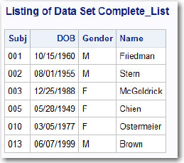
Suppose you want to add these new members to the Demographic data set and call the new data set Complete_List. Here’s how to do it using PROC SQL. (Notice that the columns are not in the same order as the Demographic data set.)
Program 26.10: Concatenating Two Tables
proc sql;
create table Complete_List as
select *
from Learn.Demographic union all corresponding
select *
from Learn.New_Members
quit;
The resulting table contains all the rows from Demographic followed by all the rows from New_Members.
Figure 26.11: Output from Program 26.10
If you leave out the keyword CORRESPONDING, here is the result (SAS log):
Figure 26.12: Resulting Log when CORRESPONDING is Omitted

If, by chance, the data types match column by column in the two data sets, SQL will perform the union. To understand this, here is another data set, New_Members_Order, where the order of the columns is changed:
Figure 26.13: Listing of New_Members_Order

Each of the four columns of New_Members_Order has the same data type (character or numeric) as the four columns of Demographic. So, if you omit the CORRESPONDING keyword when performing a union of these two data sets, you have the following result:
Figure 26.14: Result of Omitting the Keyword CORRESPONDING

You can now see why you need to choose the correct UNION operator when concatenating two data sets.
You can use functions such as MEAN and SUM to create new variables that represent means or sums of other variables. You can also create new variables within the query.
The following program shows one of the strengths of PROC SQL, which is the ability to add a summary variable to an existing table.
Suppose you want to express each person’s height in the Health data set as a percentage of the mean height of all the subjects. Using a DATA step, you would first use PROC MEANS to create a data set containing the mean height. You would then combine this with the original data set and perform the calculation. (See the section about combining detail and summary data in Chapter 10 for an example.) PROC SQL makes this task much easier. Let’s take a look.
Program 26.11: Using a Summary Function in PROC SQL
proc sql;
select Subj,
Height,
Weight,
mean(Height) as Ave_Height,
100*Height/calculated Ave_Height as
Percent_Height
from Learn.Health
quit;
The mean height is computed using the MEAN function. This value is also given the variable name Ave_Height. When you use this variable in a calculation, you need to precede it with the keyword CALCULATED, so that PROC SQL doesn’t look for the variable in one of the input data sets. Here is the result:
Figure 26.15: Output from Program 26.11

Notice how much easier this is using PROC SQL compared to a DATA step.
PROC SQL can also sort your table if you use an ORDER clause. For example, if you want the subjects in the Health table in height order, use the following:
Program 26.12: Demonstrating the ORDER Clause
title "Listing in Height Order";
proc sql;
select Subj,
Height,
Weight
from Learn.Health
order by Height;
quit;
The result (not shown) is a listing of the variables Subj, Height, and Weight in order of increasing Height.
One of the strengths of PROC SQL is its ability to create a Cartesian product. As mentioned earlier in this chapter, a Cartesian product is a pairing of every row in one table with every row in another table. Here are two tables: Demographic (used in many of the other examples in this chapter) and Insurance.
Figure 26.16: Listing of Data Sets Demographic and Insurance

You want to join (merge) these tables by Name, allowing for slight misspellings of the names. Here is an SQL query that does just that:
Program 26.13: Using PROC SQL to Perform a Fuzzy Match
title "Example of a Fuzzy Match";
proc sql;
select Subj,
Demographic.Name,
Insurance.Name
from Learn.Demographic,
Learn.Insurance
where spedis(Demographic.Name,Insurance.Name) le 25;
quit;
The SPEDIS (spelling distance) function allows for misspellings (see Chapter 12). The WHERE clause operates on every combination of names from the two tables and selects those names that are within a spelling distance of 25. In practice, you would want to compare other variables such as Gender and DOB between two files to increase the likelihood that a valid match is being made. Take a look at the listing that follows to see which names were matched by this program:
Figure 26.17: Output from Program 26.13

You could easily modify this program so that the output would not include names that match exactly.
We have only touched the surface of what you can do with SQL. Hopefully, this introduction to SQL will encourage you to learn more.
Solutions to odd-numbered problems are located at the back of this book. Solutions to all problems are available to professors. If you are a professor, visit the book’s companion website at support.sas.com/cody for information about how to obtain the solutions to all problems.
1. Use PROC SQL to list all the observations from data set Inventory where Price is greater than 20.
2. Repeat Problem 1, except use PROC SQL to create a new, temporary SAS data set (Price20) containing all observations from Inventory where the Price is greater than 20.
3. Use PROC SQL to create a new, temporary, SAS data set (N_Sales) containing the observations from Sales where Region has a value of North. Include only the variables Name and TotalSales in the new data set.
4. Data sets Inventory and Purchase are shown here:

Use PROC SQL to list all purchased items showing the Cust Number, Model, Quantity, Price, and a new variable, Cost, equal to the Price times the Quantity.
5. Data sets Left and Right are shown here. Use PROC SQL to create a new, temporary SAS data set (Both) containing Subj, Height, Weight, and Salary. Do this three ways: first, include only those subjects who are in both data sets, second, include all subjects from both data sets, and third, include only those subjects who are in data set Left.

6. Write the necessary PROC SQL statements to accomplish the same goal as the program here:
data allproducts;
set learn.inventory learn.newproducts;
run;
7. Write the necessary PROC SQL statements to accomplish the same goal as the program here:
data third;
set learn.first learn.second;
run;
Be careful! The order of the variables is not the same in both data sets. Also, some subject numbers are in both data sets.
8. Use PROC SQL to list the values of RBC (red blood cells) and WBC (white blood cells) from the Blood data set. Include two new variables in this list: Percent_RBC and Percent_WBC. These variables are the values of RBC and WBC expressed as a percentage of the mean value for all subjects. The first few observations in this list should look like this:

9. In a similar manner to Problem 8, use the Blood data set to create a new, temporary SAS data set (Percentages) containing the variables Subject, RBC, WBC, MeanRBC, MeanWBC, Percent_RBC, and Percent_WBC.
10. Run the program here to create two temporary SAS data sets, XXX and YYY.
data xxx;
input NameX : $15. PhoneX : $13.;
datalines;
Friedman (908)848-2323
Chien (212)777-1324
;
data yyy;
input NameY : $15. PhoneY : $13.;
datalines;
Chen (212)888-1325
Chambliss (830)257-8362
Saffer (740)470-5887
;
Then write the PROC SQL statements to perform a fuzzy match between the names in each data set. List the observations where the names are within a spelling distance (the SPEDIS function) of 25. The result should be only one observation, as follows:
