There are several methodologies for implementing a data warehouse or data mart that might be useful to consider when implementing QlikView in an organization. However, for me, the best approach is dimensional modeling—often called Kimball dimensional modeling—as proposed by Ralph Kimball and Margy Ross in the book The Data Warehouse Toolkit, John Wiley & Sons, now available in its third edition.
Some other methodologies, most noticeably that proposed by Bill Inmon, offer a "top-down" approach to data warehousing whereby a normalized data model is built that spans the entire enterprise, then data marts are built off this to support lines of business or specific business processes. Now, QlikView can sit very readily in this model as the data mart tool, feeding off the Enterprise Data Warehouse (EDW). However, QlikView cannot implement the normalized EDW.
In my opinion, Kimball dimensional modeling, on the other hand, is right up QlikView's street. In fact, I would suggest that you can build almost all elements of this type of data warehouse using just QlikView! The difference is that Kimball's approach is more "bottom-up"—the data marts (in our case, QlikView applications) are built first and then they can be combined to build a bigger data warehouse. Also, with this approach, we can build a data framework that power users can make use of to build their own analyses, beyond what might be achievable with other tools.
In this chapter, I am going to talk about some of the concepts of Kimball dimensional modeling, but I will not be going into deep detail on Kimball's concepts. I will describe the concept at a high level and then go in to detail on how that can be applied from a QlikView point of view. To find out more information on Kimball dimensional modeling, I recommend the following:
- Buy and read The Data Warehouse Toolkit
- Check out the Kimball Group's online resources at http://www.kimballgroup.com/data-warehouse-business-intelligence-resources
There are some key fundamental concepts that we should understand about dimensional modeling. You may already be familiar with some of the terminology. Ralph Kimball didn't create the concepts of facts and dimensions, and you will come across those terms in many contexts. However, he has created a solid methodology for modeling data in multiple different scenarios.
Essentially, facts are numbers. They are numbers that we will add up, average, count, or apply some other calculation to. For example, sales value, sales quantity, and monthly balance are all facts.
Dimensions are the values that give context to our facts. So, customer or product are both examples of dimensions. Date is also a good example of a dimension—almost every fact that you will come across will have a date context.
We store dimensions in a table of attributes. For example, a customer table might have attributes of name, city, or country. A date table will have attributes such as year, month, quarter, and week.
We will store one or many facts in a table along with the keys to associate them to the dimensions. An example of a row in a sales fact table might look like the following:
|
RowID |
DateID |
CustomerID |
ProductID |
StoreID |
Quantity |
Sales Value |
Sales Cost |
Sales Margin |
|---|---|---|---|---|---|---|---|---|
|
2345 |
20140520 |
2340000563 |
1929 |
34 |
20 |
120.00 |
100.00 |
20.00 |
What this row of data tells us is that on a particular date, in a particular store, a particular customer purchased 20 units of a particular product that had a sales value of $120.00. We can find out what product was sold by looking for ProductID 1929 in the Product dimension table.
Of course, this is not a normal query! Typically, we might start by selecting a store and then that would select for us all the fact rows that are associated with that row. We then have a calculation to add up all the sales values from that set of rows to give us the total sales for that store.
The single row in the previous fact table represents the grain of the data—the lowest level—that we are going to report on. Typically, for best results, you want the grain to be the lowest transaction level. In this case, it might not be. This customer might have bought the same product several times on the same day, so this row would actually represent an aggregated view of the data. If we added in a new field for, say, transaction number or perhaps transaction time, then we would increase the number of rows in the fact table, lowering the level of the data and changing the grain.
When we are designing the model, we need to understand what grain we want the data to be at. The business requirement will define the grain for us—if it is important for us to know the times of transactions, then we may want to have the grain at a lower level. If not, then a higher level is good. Of course, we need to consider that part of the joy of QlikView is to answer those questions that haven't been asked, so we may need to consider that, while the business does not need that grain now, they will perhaps need it in the future. We also need to balance that against the number of transaction rows in the fact table, which will be the primary driver of the size of our in-memory document and the speed of results for our users.
Once we have loaded the fact table and the four dimension tables discussed previously, our schema might look something like the following:

This structure, with one fact table and several dimension tables, with the dimensions all being at one level, is a classic star schema.
If we look at the Product table here, we will note that there is a CategoryID field and a SupplierID field. This would lead us to understand that there is additional data available for Category and Supplier that we could load and end up with a schema like the following:

This is no longer a "pure" star schema. As we add tables in this way, the schema starts to become more like a snowflake than a star—it is called a snowflake schema.
We discussed in the previous chapter about the potential issues in having many tables in a schema because of the number of joins across data tables. It is important for us to understand that it isn't necessary for the snowflake to remain and that we should actually move the data from the Category and Supplier tables into the Product table, returning to the star schema. This is not just for QlikView; it is as recommended by Kimball. Of course, we don't always have to be perfect and pragmatism should be applied.
By joining the category and supplier information into the Product table, we will restore the star schema and, from a QlikView point of view, probably improve performance of queries. The Product table will be widened, and hence the underlying data table would increase in width also, but we also have the option of dropping the CategoryID and SupplierID fields so it probably will not have a very large increase in size. As dimension tables are, generally, relatively smaller than the fact tables, any additional width in the data table will not unduly increase the size of the overall document in memory.
There are some complications with facts when it comes to the types of calculations that we can perform on them. The most basic calculation that we can do with any fact is to add up the values in that field using the Sum function. But not all facts will work correctly in all circumstances.
Luckily, most facts will probably be fully
additive. This means that we can perform a Sum function using that field and we will get a sensible and correct answer no matter what context we apply—no matter what selections we make or charts we use that calculation in. For example, the Sales Value field is usually going to be additive across all dimensions and give us a correct answer as we make different selections.
Some facts are only semi-additive. These facts can be summed, but only across some of the dimensions. For other dimensions, it does not make sense to sum them, for example, a monthly balance field. It makes sense to select a month and then sum these balances across accounts, territories, cities, and so on, but it doesn't make sense at all to sum a balance across months. If the balance in my checking account is about $100 at the end of every month, it doesn't mean that it will be $1,200 at the end of the year (though I really wish it did!).
Yet other facts won't be additive at all. These are called non-additive facts. Any ratio or percent value would not be additive. For example, if we stored the sales margin percent (the sales margin divided by the sales value) in the fact table, then this could not be sensibly added up in any way. If possible, we shouldn't have such ratios in the fact table and should, instead, always retain the original additive facts. It is perfectly sensible to calculate a margin percent expression like this in QlikView:
Sum([Sales Margin])/Sum([Sales Value])
Because both of the facts involved are additive, the expression will calculate correctly across all dimensions.
There are a few different types of fact tables that we will encounter reasonably regularly. These are as follows:
- Transaction
- Periodic snapshot
- Factless
The following sections give a brief description of these and how you may need to deal with them in QlikView.
The transaction fact table is by far the most common type that you will encounter. At the lowest grain, each row in the table represents one event that has happened; for example, a sale of a particular product in a particular store to a particular customer at a particular time by a particular operator at a particular till. Another example might be the scanning of a product as it is placed into a pick basket in a warehouse automated pick system.
Each of these is an atomic event—it is the lowest level of detail that we can have about the process in question. It also gives us more flexibility from a QlikView point of view in that we can calculate our results over many different dimensions.
Because this transaction represents one event, there are generally relatively few facts associated with it. We might, for example, just have quantity and value. If the system gives us the information, we might also have cost and perhaps a derived margin, but that would be all.
We can, as we have already discussed, aggregate transactions to a higher level. If the retailer does not care about which customer bought a product or at what till, we might remove the customer, till, time, and operator from the transaction and then roll up the values to just date, store, and product, summing up the facts appropriately.
Often, this is done for a performance benefit because less rows will equal less memory used by QlikView. However, when we change the grain and reduce the number of dimensions, we also have the opportunity to add other facts to the table from other events. For example, retailers often throw out unsaleable items—this is called waste. This event would also have a date, store, and product associated with it so we could join the two fact tables to create a new, wider fact table. Any other events in the store that have a date and product associated with them could equally be joined in.
The fact tables are called periodic snapshot fact tables. Usually they have a period associated with them such as a particular day or rolled up to week or month.
In the previous example, the periodic snapshot table will have the same structure as a transaction fact table and it is fair to say that it still counts as a transaction fact table for modeling purposes. The facts are rolled up from the underlying facts and can be treated the same. However, there are periodic snapshot tables that will represent the end of period position for a value—for example, an account balance or an inventory level—and we need to be careful with these because the facts will be semi-additive.
There are fact tables that record an atomic event that doesn't have any particular amount or other measure associated with it. For example, many retailers will have a person on the shop floor who has the task of wandering around checking for empty shelves. If they find a shelf where all the stock has been sold, they scan the product bar code off the shelf and this goes into the backend system. This "gap count" just records the date, time, shelf number, and product. There is no quantity or value involved.
Quite often, we will create a fact—usually just with a value of 1—to be used in calculations.
Because QlikView isn't too hung up on referential integrity of data, we as designers should always be thinking about it because we shouldn't really allow a disconnect between dimension tables and fact tables. Null values in fact fields are not a problem for QlikView. They will get completely ignored in the majority of calculations, and this is the correct behavior that we want.
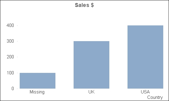
Null values in dimension keys are a different matter. QlikView will allow them, but this causes us a problem when it comes to charts. Let's look at a very simple example:
Dimension:
Load * Inline [
CustomerID, Customer, Country
1, Customer A, USA
2, Customer B, USA
3, Customer C, UK
4, Customer D, UK
];

Fact:
Load
*
Inline [
Date, CustomerID, Sales Value
2014-01-01, 1, 100
2014-01-01, 2, 100
2014-01-01, 3, 100
2014-01-01, 4, 100
2014-01-01, , 100
2014-01-02, 1, 100
2014-01-02, 2, 100
2014-01-02, 4, 100
];
If we create a chart for the sum of sales value by country, it will look like the following:

We have a bar that shows an amount associated with a null value. We can't select this bar to find out any other information. I can't drill down to discover the transactions that are not associated to a country.
The way to handle this is to actually create an additional row in the dimension table with a default value and key that we can use in the fact table:
Dimension:
Load * Inline [
CustomerID, Customer, Country
0, Missing, Missing
1, Customer A, USA
2, Customer B, USA
3, Customer C, UK
4, Customer D, UK
];

Fact:
Load
   Date,
   If(Len(CustomerID)=0, 0, CustomerID) As CustomerID,
   [Sales Value]
Inline [
Date, CustomerID, Sales Value
2014-01-01, 1, 100
2014-01-01, 2, 100
2014-01-01, 3, 100
2014-01-01, 4, 100
2014-01-01, , 100
2014-01-02, 1, 100
2014-01-02, 2, 100
2014-01-02, 4, 100
];
We now have a value in the Country field that we can drill into to discover fact table rows that do not have a customer key:
There may actually be cases where the key is not missing but is just not applicable. In that case, we can add an additional "Not Applicable" row to the dimension table to handle that situation.
We have a good idea now about fact tables, but we have only briefly talked about the dimension tables that create the context for the facts.
We discussed star schemas previously, and we discussed that snowflake schemas are not ideal for QlikView and also not recommended by Kimball.
Snowflaking dimensions is akin to the normalization process that is used to design transactional databases. While it may be appropriate for transactional databases, where insert speed is the most important thing, it is not appropriate for reporting databases, where retrieval speed is the most important thing. So denormalizing the dimension tables, by joining the lower level tables back into the main table (joining category and supplier into product in the previous example), is the most efficient method—and this applies for QlikView as well as any database warehouse.
There is another excellent reason for creating a single table to represent a dimension. We are generally not going to build only one QlikView document. We will probably have many business processes or areas that we will want to cover with our applications. These QlikView documents might share dimensions, for example, both a sales and a purchases application will have a product dimension. Depending on the organization, the product that you buy might be the same as the products that you sell. Therefore, it makes sense to build one product dimension, store it to QVD, and then use it in any documents that need it.
Dimensions created that will be shared across multiple dimensional models are called conformed dimensions.
In Kimball dimensional modeling, there is the concept of replacing the original primary key values of dimensions, in both the dimension and fact tables, with a sequential integer value. This should especially be the case where the primary key is made up of multiple key values.
We should recognize this immediately in QlikView as we already discussed it in Chapter 1, Performance Tuning and Scalability—we use the AutoNumber function to create a numeric key to associate the dimension with the fact table.
If necessary, we can retain the original key values in the dimension table so that they can be queried, but we do not need to retain those values in the fact table.
A late arriving dimension value is a value that does not make it into the dimension table at the time that we load the information into QlikView. Usually, this is a timing issue. The symptoms are the same as if the dimension value doesn't exist at all—we are going to have a referential integrity issue.
Let's look at a quick example:
Dimension:
Load * Inline [
CustomerID, Customer, Country
1, Customer A, USA
2, Customer B, USA
3, Customer C, UK
4, Customer D, UK
];

Fact:
Load * Inline [
Date, CustomerID, Sales Value
2014-01-01, 1, 100
2014-01-01, 2, 100
2014-01-01, 3, 100
2014-01-01, 4, 100
2014-01-01, 5, 100
2014-01-02, 1, 100
2014-01-02, 2, 100
2014-01-02, 4, 100
];
We can see that we have four rows in the dimension table, but we have five distinct key values in the fact table. We need to add additional rows to the dimension table derived from the fact table:
Concatenate (Dimension)
Load Distinct
   CustomerID,
   'Missing ' & CustomerID As Customer,
   'Missing ' & CustomerID As Country
Resident
   Fact
Where Len(Lookup('CustomerID', 'CustomerID', CustomerID, 'Dimension'))=0;
You might wonder why I am not using a Not Exists function here. Exists will check in the symbol table to see whether a value has already been loaded. We only have one symbol table per field and, in this case, both tables have the same field name—CustomerID—and hence will have the same symbol table. Because the fact table has been loaded, the symbol table will be fully loaded with all of the available values, so a Not Exists function will never return true and no additional values will be loaded.
Now that we know a bit more about the definitions around facts and dimensions, we can talk about Kimball's dimensional design process. This, as a basic tenet, can be applied to almost every QlikView application that you might build.
The four steps are as follows:
- Select the business process
- Declare the grain
- Identify the dimensions
- Identify the facts
There are often two ways that developers choose to pick the subject of their QlikView documents. One is line-of-business—for example, Sales, HR, Finance, and so on. The other is by business process. A business process is a set of activities that a business performs that may generate a set of metrics, for example, process orders, ship orders, or order stock. Each process will generate one set of facts.
The difference between a line-of-business application and a process-based application is sometimes so subtle that you'll feel there isn't really a difference at all! This is especially true where the identified line-of-business appears to only really have one process within an organization.
Take selling for example. In some organizations, the only thing that is important about selling is the taking orders process. If you are asked to build a sales application for that organization, the line-of-business and the process will be the same. In other organizations, however, they will also be looking for information on customer and prospect contacts—visits, phone calls, and so on.
The line-of-business application will probably want to try and load the facts from both processes so as to compare them and answer business questions about the relationship between visits and orders. The process-based application will tend to just focus on the one set of facts.
In a "pure" Kimball dimensional model, we focus on the process model and one fact table. Where we are building a more line-of-business application with multiple fact tables, we should apply this four step sequence for each process. We will discuss later how we handle a QlikView model with multiple fact tables.
So, the first step is to select that business process.
We have already learned what is meant by grain—the level of detail in the fact table. By declaring the grain, we are specifying what level of aggregation we want to deal with.
In almost every situation, the best choice of grain is the atomic choice—the transactional data at the lowest level of detail. Going atomic means that our users can slice and dice the information by whatever dimensions they want. By making a choice to aggregate the fact table, we remove some choice from the user. For example, if we aggregate the retail sales to day, store, and product, we remove the ability of the users to interrogate the data by till, operator, or time of day.
The dimensions that will be used will pretty much fall out of grain declaration. The complication here is where we are doing a line-of-business app; while we are doing this step by step for one process at a time, we need to be aware of those dimensions that are shared, and we should be sure to have a conformed dimension.
There are a couple of things that you will come up against repeatedly in creating QlikView documents. One that you will pretty much use in all QlikView documents is the creation of a calendar dimension. Another, that you might not use in every application but will come in useful, is dealing with hierarchies. Lastly, we will look at the practice of creating dimensional facts.
Almost every fact table that we will come across will have a date of some sort—at least one, there may be more. Quite often, the source system that we will be extracting the data from may have a calendar table that we can use as the dimension table, but sometimes it doesn't and we need to derive one ourselves.
The basic idea of creating a calendar dimension is to first establish the bounds—what are the earliest and latest dates that should be included. Once we have that, we can generate a row for every date between those bounds (inclusive) and use QlikView functions to derive the date parts—year, month, week, and so on.
In training, you may have come across some methods to establish the minimum and maximum values of the date by querying the fact table. For example, you may have seen something like the following:
MinMaxDates:
Load
   Min(OrderDate) As MinDate,
   Max(OrderDate) As MaxDate
Resident
   Fact;

Let vStartDate=Peek('MinDate');
Let vEndDate=Peek('MaxDate');

Drop Table MinMaxDates;
There are some problems with this method, so I rarely use it outside the classroom.
One of them is that once you get past a million fact table records, the time taken to calculate the min and max values becomes more and more perceptible and unacceptable in a well-designed script.
However, for me, the main issue is that it is a pointless exercise. The minimum date will rarely, if ever, change—it is a well-known value and can therefore be stated in the script without having to try and calculate it every time. The maximum date, depending on the business, is almost always going to be today, yesterday, or some derivation thereof. Therefore, it is easily calculable without having to scan down through a data table. My calendar script is almost always going to start off something like the following:
Let vStartDate=Floor(MakeDate(2009,1,1));
Let vEndDate=Floor(Today());
Let vDiff=vEndDate-vStartDate+1;
So, I am stating that the first date for my data is January 1, 2009. The end date is today. When working with dates, I will always transform them to integer values, especially when used with variables. Integers are a lot easier to deal with. I will also always calculate the number of dates that I will need in my calendar as the last date minus the first date plus 1. The rest of my script might look like the following:
Calendar:
Load *,
   Date(MonthStart(DateID), 'YYYY-MM') As YearMonth,
   Year & '-' & Quarter As YearQuarter,
   WeekYear & '-' & Num(Week, '00') As YearWeek;
Load
   DateID,
   Year(DateID) As Year,
   Month(DateID) As Month,
   Date(DateID) As Date,
   Day(DateID) As Day,
   Week(DateID) As Week,
   'Q' & Ceil(Month(DateID)/3) As Quarter,
   WeekYear(DateID) As WeekYear,
   -Year2Date(DateID) As YTD_Flag,
   -Year2Date(DateID, -1) As LYTD_Flag;
Load
   RecNo()-1+$(vStartDate) As DateID
AutoGenerate($(vDiff));
There are a couple of preceding loads here, which I quite like to use to make scripts more readable. If you haven't come across preceding loads, any load statement that is just a list of field names and functions, terminated with a semicolon, will load its data from the next statement down in the script.
In this case, at the bottom of the pile is an AutoGenerate function that will generate the required number of rows. We use a calculation based on the current record number and the start date to calculate the correct date that we should use. The preceding load directly above it will create all the date parts—year, month, week, and so on, and a couple of year-to-date flags that we can use in calculations. The topmost preceding load will use fields created in the middle part to create additional fields.
If you really need a script to derive the calendar table from the data, I can highly recommend the script published on the Qlik community website by Torben Seebach from itelligence in Denmark at http://community.qlik.com/docs/DOC-6662.
Way back in the day, there was a piece of script going around that would unwrap a hierarchical relationship in data. It was the most complicated piece of script that you could imagine—but it worked. It was so popular that Qlik decided to create new functions in QlikView to do the operation. There are two—Hierarchy and HierarchyBelongsTo.
The Hierarchy function will unwrap the hierarchy and create multiple leaf nodes for each level of the hierarchy. Let's create a very simple hierarchical table:
Load * Inline [
NodeID, Location, ParentID
1, World,
2, EMEA, 1
3, Americas, 1
4, AsiaPac, 1
5, USA, 3
6, Canada, 3
7, Brazil, 3
8, UK, 2
9, Germany, 2
10, France, 2
11, China, 4
12, Japan, 4
13, New York, 5
14, Texas, 5
15, California, 5
16, London, 8
17, Greater Manchester, 8
18, Manchester, 17
19, Bavaria, 9
20, Munich, 19
21, New York, 13
22, Heuston, 14
23, San Francisco, 15
];
Each row has a node key, a name, and a parent key that refers to the node key of the level above. So, USA's parent key is 3, which refers to the node key of the Americas.
The first three parameters of the Hierarchy function are mandatory. The other parameters are optional. The parameters are as follows:
We don't need to have the path or the depth fields created, but they can be useful to have.
To change the preceding table into a full hierarchy, we add the Hierarchy statement above the Load statement:
Hierarchy(NodeID, ParentID, Location, 'Parent Location', 'Location', 'PathName', '~', 'Depth')
Load * Inline [
...
This will produce a table that looks like the following:

If the PathName field is added as a listbox, the Show as TreeView option can be specified on the General properties tab:

With this option turned on, the listbox will be presented in a tree view:

The HierarchyBelongsTo function is slightly different in that it unwraps the link from parent to child and makes it navigable in QlikView. Each child node is associated with its parent, grandparent, and so on. We can also create a field to capture the depth difference between node and ancestor.
The parameters are as follows—only the DepthDiff parameter is optional:
Taking the inline table of the previous locations, we can replace the Hierarchy function with a HierarchyBelongsTo function as shown:
HierarchyBelongsTo (NodeID, ParentID, Location, 'AncestorID', 'AncestorName', 'DepthDiff')
Load * Inline [
...
Then, we will obtain a table that looks like the following:

This table has all the nodes associated to their parents and vice versa.
Most of the facts that we deal with in the fact table are numbers that we will calculate and recalculate based on a user's selections. It can sometimes be useful for us to precalculate some values in the script that are less dependent on other dimensions and store them in the dimension table. Some examples are:
- Customer balance
- Number of orders this year
- Number of orders last year
- Current stock quantity
These values should all be calculable from the fact table, but having them precalculated in the dimension table means that performance can be improved. Having them in the dimension table also makes them easier to use as dimension type values—we can query and group by them.
Creating these facts in the script is as simple as loading and grouping from the fact table, for example:
Left Join (Customer)
Load
   CustomerID,
   Count(OrderID) As [Orders This Year],
   Sum([Line Value]) As [Sales This Year]
Resident Fact
Where Year(OrderDate)=Year(Today())
Group by CustomerID;