Chapter 9: Training ML Models at Scale in SageMaker Studio

A typical ML life cycle starts with prototyping and will transition to a production scale where the data gets larger, models get more complicated, and the runtime environment gets more complex. Getting a training job done requires the right set of tools. Distributed training using multiple computers to share the load addresses situations that involve large datasets and large models. However, as complex ML training jobs use more compute resources, and more costly infrastructure (such as Graphical Processing Units (GPUs)), being able to effectively train a complex ML model on large data is important for a data scientist and an ML engineer. Being able to see and monitor how a training script interacts with data and compute instances is critical to optimizing the model training strategy in the training script so that it is time- and cost-effective. Speaking of cost when training at a large scale, did you know you can easily save more than 70% when training models in SageMaker? SageMaker Studio makes training ML models at scale easier and cost-effective.

In this chapter, we will be learning about the following:

• Performing distributed training in SageMaker Studio
• Monitoring model training and compute resources with SageMaker Debugger
• Managing long-running jobs with check-pointing and spot training

Technical requirements

For this chapter, you need to access the code provided at https://github.com/PacktPublishing/Getting-Started-with-Amazon-SageMaker-Studio/tree/main/chapter09.

Performing distributed training in SageMaker Studio

As the field of deep learning advances, ML models and training data are growing to a point that one single device is no longer sufficient for conducting effective model training. The neural networks are getting deeper and deeper, and gaining more and more parameters for training:

• LeNet-5, one of the first Convolutional Neural Network (CNN) models proposed in 1989 that uses 2 convolutional layers and 3 dense layers, has around 60,000 trainable parameters.
• AlexNet, a deeper CNN architecture with 5 layers of convolutional layers and 3 dense layers proposed in 2012, has around 62 million trainable parameters.
• Bidirectional Transformers for Language Understanding (BERT), a language representation model using a transformer proposed in 2018, has 110 million and 340 million trainable parameters in the base and large models respectively.
• Generative Pre-trained Transformer 2 (GPT-2), a large transformer-based generative model proposed in 2019, has 1.5 billion trainable parameters.
• GPT-3 is the next version, proposed in 2020, that reaches 175 billion trainable parameters.

Having more parameters to train means that there is a larger memory footprint during training. Additionally, the training data size needed to fit a complex model has also gone up significantly. For computer vision, one of the most commonly used training datasets, ImageNet, has 1.2 million images. For Natural Language Processing (NLP), GPT-3 is trained with 499 billion tokens, for example.

However, the latest and greatest GPU device would still struggle to hold up for such training requirements. The latest GPU device from NVIDIA, the A100 Tensor Core GPU available on AWS P4d.24xlarge instances, has 40 GB of GPU memory, but it would not be sufficient to hold the GPT-3 model, which has 175 billion parameters, as such a network would need 175 x 109 x 4 bytes = 700 GB when using the FP32 precision. Therefore, developers are going beyond single GPU device training and resorting to distributed training – that is, training using multiple GPU devices and multiple compute instances.

Let's understand why and how distributed training helps.

Understanding the concept of distributed training

In ML model training, the training data is fed into the loss optimization process in order to compute the gradients and weights for the next step. When data and parameters are much larger, as in the case of deep learning, having a full dataset that fits into the optimization becomes less feasible due to the GPU memory available on the device. It is common to use the stochastic gradient descent optimization approach, which estimates the gradients with a subset (batch size) of the full training dataset in each step, to overcome the GPU memory limitation. However, when a model or each data point is too large to have a meaningful batch size for the model training, we will not be able to converge to an optimal, accurate model in a reasonable timeframe.

Distributed training is a practice to distribute parts of the computation to multiple GPU devices and multiple compute instances (also called nodes), and synchronize the computation from all devices before proceeding to the next iteration. There are two strategies in distributed training: data parallelism and model parallelism.

Data parallelism distributes the training dataset during epochs from disk to multiple devices and instances while each device contains a portion of data and a complete replica of the model. Each node performs a forward and backward propagation pass using different batches of data and shares trainable weight updates with other nodes for synchronization at the end of a pass. With data parallelism, you can increase the batch size by n-fold, where n is the number of GPU devices across nodes. An appropriately large batch size allows better generalization during the estimation of gradients and also reduces the number of steps needed to run through the entire pass (an epoch).

Note

It has also been observed in practice that an overly large batch size will hurt the quality and generalization of a model. This is model- and dataset-dependent and requires experimentations and tuning to find out an appropriate batch size.

Data parallelism is illustrated in Figure 9.1:

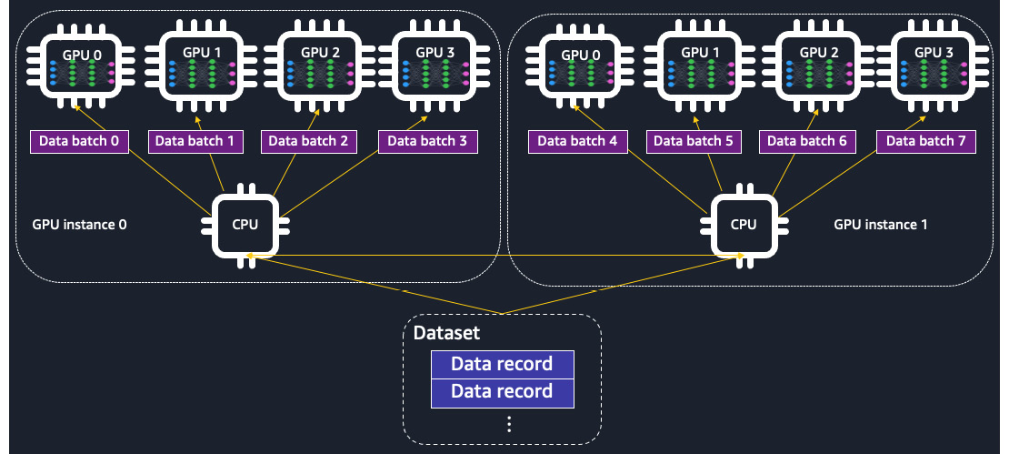
Figure 9.1 – The training data is distributed across GPU devices in data parallelism. A complete replica of the model is placed on each GPU device

Alternatively, model parallelism distributes a large model across nodes. Partitioning of a model is performed at a layers and a weights level. Each node possesses a partition of the model. Forward and backward propagations take place as a pipeline, with the data batches going through the model partitions on all nodes before the weight updates. To be more specific, each data batch is split into micro-batches and feeds into each part of the model, located on devices for forward and backward passes. With model parallelism, you can more effectively train a large model that needs a higher GPU memory footprint than a single GPU device using memory collectively from multiple GPU devices. Model parallelism is illustrated in Figure 9.2:

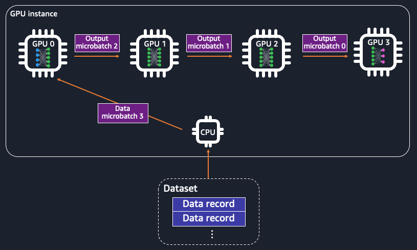
Figure 9.2 – The model is partitioned across GPU devices in model parallelism. The training data is split into micro-batches and fed into the GPUs, each of which has a part of the model as a pipeline

When should we use data parallelism or model parallelism? It depends on the data size, batch, and model sizes in training. Data parallelism is suitable for situations when a single data point is too large to have a desirable batch size during training. The immediate trade-off of having a small batch size is having a longer runtime to finish an epoch. You may want to increase the batch size so that you can complete an epoch under a reasonable timeframe. You can use data parallelism to distribute a larger batch size to multiple GPU devices. However, if your model is large and takes up most GPU memory in a single device, you will not enjoy the scale benefit of data parallelism much. This is because, in data parallelism, an ML model is fully replicated onto each of the GPU devices, leaving little space for any data. You should use model parallelism when you have a large model in relation to the GPU memory.

SageMaker makes running distributed training for large datasets and large models easy in the cloud. SageMaker's distributed training libraries support data parallelism and model parallelism for the two most popular deep learning frameworks, TensorFlow and PyTorch, when used in SageMaker. SageMaker's distributed data parallel library scales your model training with near-linear scaling efficiency, meaning that the reduction in training time in relation to the number of nodes is close to linear. SageMaker's distributed model parallel library automatically analyzes your neural network architecture and splits the model across GPU devices and orchestrates the pipeline execution efficiently.

In the following sections, we'll learn how we can implement data parallelism and model parallelism in SageMaker Studio for our training scripts written in TensorFlow and PyTorch.

Note

Both TensorFlow and PyTorch are supported by the two distributed training libraries. The distributed training concepts remain the same between the two deep learning frameworks. We will focus on TensorFlow for the data parallel library and PyTorch for the model parallel library.

The data parallel library with TensorFlow

SageMaker's distributed data parallel library implements simple APIs that look similar to TensorFlow's way of performing model training in a distributed fashion but conduct distributed training that is optimized with AWS's compute infrastructure. This means that you can easily adopt SageMaker's API without making sophisticated changes to your existing distributed training code written in TensorFlow. If this is your first model training with distribution, we will demonstrate the modification needed to adapt SageMaker's distributed data parallel library to your existing model training script.

Let's go to SageMaker Studio and start working with the Getting-Started-with-Amazon-SageMaker-Studio/chapter09/01-smdp_tensorflow_sentiment_analysis.ipynb notebook. This example is built on top of the training example we walked through in Chapter 5, Building and Training ML Models with the SageMaker Studio IDE (Getting-Started-with-Amazon-SageMaker-Studio/chapter05/02-tensorflow_sentiment_analysis.ipynb), where we trained a deep learning model using the TensorFlow Keras API on an IMDB review dataset. Back in Chapter 5, Building and Training ML Models with SageMaker Studio IDE, we ran the training script on one ml.p3.2xlarge instance, which only has one NVIDIA Tesla V100 GPU. Now, in this chapter, we will use SageMaker's distributed data parallel library to extend the code to work with multiple GPU devices, either from an instance or from multiple instances. And remember that we can always easily specify the number of instances and the type of the instances in the sagemaker.tensorflow.TensorFlow estimator. Let's open the notebook and select the Python 3 (TensorFlow 2.3 Python 3.7 CPU Optimized) kernel and an ml.t3.medium instance, and run the first six cells to prepare the SageMaker session and the dataset. The cell leading with %%writefile code/smdp_tensorflow_sentiment.py is where modification to adopt the distributed training script will go. Follow the next steps to see the changes that need to be made to enable the distributed data parallel library:

1. First, import the TensorFlow module of the data parallel library:

   import smdistributed.dataparallel.tensorflow as sdp

2. After the library is imported, we need to initialize the SageMaker distributed data parallel library in order to use it during runtime. We can implement it right after the import statements or in main (if __name__ == "__main__"):

   sdp.init()

3. Then, we discover all the GPU devices available in the compute instance fleet and configure the GPUs so that they are aware of the ranking within an instance. If an instance has eight GPU devices, each of them will get assigned a rank from zero to seven. The way to think about this is that each GPU device establishes a process to run the script and gets a unique ranking from sdp.local_rank():

   gpus = tf.config.experimental.list_physical_devices('GPU')

   if gpus:

       local_gpu = gpus[sdp.local_rank()]

       tf.config.experimental.set_visible_devices(local_gpu, 'GPU')

4. We also configure the GPUs to allow memory growth. This is specific to running TensorFlow with the SageMaker distributed data parallel library:

   for gpu in gpus:

       tf.config.experimental.set_memory_growth(gpu, True)

The compute environment is now ready to perform distributed training.

5. We scale the learning rate by the number of devices. Because of data parallelism, we will be able to fit in a larger batch size. With a larger batch size, it is recommended to scale the learning rate proportionally:

   args.learning_rate = args.learning_rate * sdp.size()

6. Previously in Chapter 5, Building and Training ML Models with SageMaker Studio IDE, we trained the model using Keras' model.fit() API, but we have to make some changes to the model training. SageMaker's distributed data parallel library does not yet support Keras' .fit() API and only works with TensorFlow core modules. To use SageMaker's distributed data parallel library, we can use the automatic differentiation (tf.GradientTape) and eager execution from TensorFlow 2.x. After defining the model using Keras layers in the get_model() function, instead of compiling it with an optimizer, we write the forward and backward pass explicitly with the loss function, the optimizer, and also the accuracy metrics defined explicitly:

   model = get_model(args)

   loss = tf.losses.BinaryCrossentropy(name = 'binary_crossentropy')

   acc = tf.metrics.BinaryAccuracy(name = 'accuracy')

   optimizer = tf.optimizers.Adam(learning_rate = args.learning_rate)

   with tf.GradientTape() as tape:

       probs = model(x_train, training=True)

       loss_value = loss(y_train, probs)

       acc_value = acc(y_train, probs)

We then wrap tf.GradientTape with SMDataParallel's DistributedGradientTape to optimize the AllReduce operation during the multi-GPU training. AllReduce is an operation that reduces the matrixes from all distributed processes:

tape = sdp.DistributedGradientTape(tape, sparse_as_dense = True)

Note that the sparse_as_dense argument is set to True because we have an embedding layer in the model that will generate a spare matrix.

7. At the start of the training, broadcast the initial model variables from the head node (rank 0) to all other worker nodes (rank 1 onward). We use a first_batch variable to denote the start of the training epochs:

   if first_batch:

       sdp.broadcast_variables(model.variables, root_rank=0)

       sdp.broadcast_variables(optimizer.variables(), root_rank=0)

8. Average the loss and accuracy across devices; this process is called all-reduce:

   loss_value = sdp.oob_allreduce(loss_value)

   acc_value = sdp.oob_allreduce(acc_value)

9. Put these steps in a training_step() function to perform a forward and backward pass, decorated with @tf.function. Run this training step in a nested for loop to go over epochs and batches of training data. We need to make sure that all GPU devices are getting an equal amount of data during a pass. We do this by taking data that is divisible by the total number of GPU devices in the inner for loop:

   train_dataset.take(len(train_dataset)//sdp.size())

10. After the training epoch loop, we save the model, only using the leader device:

    if sdp.rank() == 0:

        model.save(os.path.join(args.model_dir, '1'))

11. Last but not least in the training script, we convert the training data into a tf.data.Dataset object and set up the batching in the get_train_data() function so that it will work with our eager execution implementation. Note that we need drop_remainder to prevent the dataset from being of an equal batch_size across devices:

    dataset = tf.data.Dataset.from_tensor_slices((x_train, y_train))

    dataset = dataset.batch(batch_size, drop_remainder=True)

12. We then move on to SageMaker's TensorFlow estimator construct. To enable the SageMaker distributed data parallel library in a training job, we need to provide a dictionary:

    distribution = {'smdistributed': {'dataparallel': {'enabled': True}}}

This is given to the estimator, as follows.

train_instance_type = 'ml.p3.16xlarge'

estimator = TensorFlow(source_dir='code',

     entry_point='smdp_tensorflow_sentiment.py',

     ...

     distribution=distribution)

Also, we need to choose a SageMaker instance from the following instance types that supports SageMaker's distributed data parallel library: ml.p4d.24xlarge, ml.p3dn.24xlarge, and ml.p3.16xlarge:

1. The ml.p4d.24xlarge instance equips with 8 NVIDIA A100 Tensor Core GPUs, each with 40 GB of GPU memory.
2. The ml.p3dn.24xlarge instance comes with 8 NVIDIA Tesla V100 GPUs, each with 32 GB of GPU memory.
3. The ml.p3.16xlarge instance also comes with 8 NVIDIA Tesla V100 GPUs, each with 16 GB of GPU memory.

For demonstration purposes, we will choose ml.p3.16xlarge, which is the least expensive one among the three options. One single ml.p3.16xlarge is sufficient to run distributed data parallel training in SageMaker, as there will be 8 GPU devices to perform the training.

As there are more GPU devices and GPU memory to carry out the batching in an epoch, we can now increase batch_size. We scale batch_size 8 times from what we used in Chapter 5, Building and Training ML Models with SageMaker Studio IDE – that is, 64 x 8 = 512.

13. With the estimator, we can proceed to call estimator.fit() to start the training.

To verify that the training is run with multiple GPU devices, the simplest way to tell is from the standard output. You can see a prefix of [x, y]<stdout>: message being added to indicate the process ranking from which the message is produced, as shown in Figure 9.3. We will learn more about this topic in the Monitoring model training and compute resource with SageMaker Debugger section:

Figure 9.3 – The standard output from the cell, showing messages printed from process ranks – [1,0] to [1,7]. In our example, we use one ml.p3.16xlarge instance that has eight GPU devices

Even though here I am not using PyTorch to demonstrate SageMaker's distributed data parallel library, PyTorch is indeed supported by the library under the smdistributed.dataparallel.torch module. This module has a set of APIs that are similar to PyTorch's native distributed data parallel library. This means that you do not require many coding changes to adopt SageMaker's distributed data parallel library for PyTorch, which is optimized for training using SageMaker's infrastructure. You can find more details on how to adopt it in your PyTorch scripts at https://docs.aws.amazon.com/sagemaker/latest/dg/data-parallel-modify-sdp-pt.html.

In the next section, we will run a PyTorch example and adopt model parallelism.

Model parallelism with PyTorch

Model parallelism is particularly useful when you have a large network model that does not fit into the memory of a single GPU device. SageMaker's distributed model parallel library implements two features that enable efficient training for large models so that you can easily adapt the library to your existing training scripts:

• Automated model partitioning, which maximizes GPU utilization, balances the memory footprint, and minimizes communication among GPU devices. In contrast, you can also manually partition the model using the library.
• Pipeline execution, which determines the order of computation and data movement across parts of the model that are on different GPU devices. There are two pipeline implementations: interleaved and simple. An interleaved pipeline prioritizes the backward passes whenever possible. It uses GPU memory more efficiently and minimizes the idle time of any GPU device in the fleet without waiting for the forward pass to complete to start the backward pass, as shown in Figure 9.4:

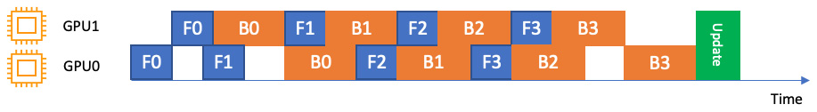
Figure 9.4 – An interleaved pipeline over two GPUs (GPU0 and GPU1). F0 represents a forward pass for the first micro-batch and B1 represents a backward pass for the second micro-batch. Backward passes are prioritized whenever possible

A simple pipeline, on the other hand, waits for the forward pass to complete before starting the backward pass, resulting in a simpler execution schedule, as shown in Figure 9.5:

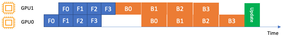
Figure 9.5 – A simple pipeline over two GPUs. Backward passes are run only after the forward passes finish

Note

Images in Figure 9.4 and 9.5 are from: https://docs.aws.amazon.com/sagemaker/latest/dg/model-parallel-core-features.html

Let's start an example with the notebook in chapter09/02-smmp-pytorch_mnist.ipynb, where we are going to apply SageMaker's distributed model parallel library to train a PyTorch model to classify digit handwriting using the famous MNIST digit dataset. Open the notebook in SageMaker Studio and use the Python 3 (Data Science) kernel and an ml.t3.medium instance:

1. As usual, set up the SageMaker session and import the dependencies in the first cell.
2. Then, create a model training script written in PyTorch. This is a new training script. Essentially, it is training a convolutional neural network model on the MNIST handwriting digit dataset from the torchvision library. The model is defined using the torch.nn module. The optimizer used is the AdamW optimization algorithm. We implement the training epochs and batching, as it allows us to have the most flexibility to adopt SageMaker's distributed model parallel library.
3. SageMaker's distributed model parallel library for PyTorch can be imported from smdistributed.modelparallel.torch:

   import smdistributed.modelparallel.torch as smp

4. After the library is imported, initialize the SageMaker distributed model parallel library in order to use it during runtime. We can implement it right after the import statements or in main (if __name__ == "__main__"):

   smp.init()

5. We will then ping and set the GPU devices with their local ranks:

   torch.cuda.set_device(smp.local_rank())

   device = torch.device('cuda')

6. The data downloading process from torchvision should only take place in the leader node (local_rank = 0), while all the other processes (on other GPUs) should wait until the leader node completes the download:

   if smp.local_rank() == 0:

       dataset1 = datasets.MNIST('../data', train=True,

                     download=True, transform=transform)        

   smp.barrier() # Wait for all processes to be ready

7. Then, wrap the model and the optimizer with SageMaker's distributed model parallel library's implementations:

   model = smp.DistributedModel(model)

   optimizer = smp.DistributedOptimizer(optimizer)

Up to now, the implementation between SageMaker's distributed data parallel library and model parallel library has been quite similar. The following is where things get different for the model parallel library.

8. We create a train_step() for function forward and backward passes and decorate it with @smp.step:

   @smp.step

   def train_step(model, data, target):

       output = model(data)

       loss = F.nll_loss(output, target, reduction='mean')

       model.backward(loss)

       return output, loss

Create another train() function to implement the batching within an epoch. This is where we call train_step() to perform the forward and backward passes for a batch of data. Importantly, the data-related to.(device) calls need to be placed before train_step() while the typical model.to(device) is not required. Placing the model to a device is done automatically by the library.

Before stepping to the next batch, we need to average the loss across micro-batches with .reduce_mean(). Also, note that optimizer.step() needs to take place outside of train_step():

def train(model, device, train_loader, optimizer, epoch):

    model.train()

    for batch_idx, (data, target) in enumerate(train_loader):

        data, target = data.to(device), target.to(device)

        optimizer.zero_grad()

        _, loss_mb = train_step(model, data, target)

        # Average the loss across microbatches.

        loss = loss_mb.reduce_mean()

        optimizer.step()

9. Implement test_step(), decorated with @smp.step, and test() similarly for model evaluation. This allows model parallelism in model evaluation too.
10. After the epochs loop, save the model with smp.dp_rank()==0 to avoid data racing and ensure the gathering happens properly. Note that we set partial=True if we want to be able to load the model later and further train it:

    if smp.dp_rank() == 0:

        model_dict = model.local_state_dict()

        opt_dict = optimizer.local_state_dict()

        model = {'model_state_dict': model_dict, 'optimizer_state_dict': opt_dict}

        model_output_path = f'{args.model_dir}/pt_mnist_checkpoint.pt'

        smp.save(model, model_output_path, partial=True)

11. We then move on to the SageMaker PyTorch estimator construct. To enable SageMaker's distributed model parallel library in a training job, we need to provide a dictionary to configure SageMaker's distributed model parallel library and the Message Passing Interface (MPI). SageMaker's distributed model parallel library uses the MPI to communicate across nodes, so it needs to be enabled. The following snippet instructs SageMaker to partition the model into two 'partitions': 2, to optimize for speed when partitioning the model 'optimize': 'speed', to use a micro-batch of four 'microbatches': 4, to employ an interleaved pipeline schedule ('pipeline': 'interleaved'), and to disable distribute data parallel 'ddp': False. The MPI is enabled with four processes per host 'mpi':{'enabled': True, 'processes_per_host': 2}}, which should be smaller than or equal to the number of GPU devices:

    distribution = {'smdistributed': {

                        'modelparallel': {

                            'enabled': True,

                            'parameters': {

                                'partitions': 2,

                                 'optimize': 'speed',

                                'microbatches': 4,

                                'pipeline': 'interleaved',

                                'ddp': False

                            }

                        }

                    },

                    'mpi': {

                        'enabled': True,

                        'processes_per_host': 2

                    }

                }

You can find the full list of parameters for distribution at https://sagemaker.readthedocs.io/en/stable/api/training/smd_model_parallel_general.html#smdistributed-parameters.

12. We then apply the distribution dictionary to the PyTorch estimator and use one ml.p3.8xlarge instance, which has four NVIDIA Tesla V100 GPUs. Unlike SageMaker's distributed data parallel library, SageMaker's distributed model parallel library is supported by all instances with multiple GPU devices.
13. We can then proceed to call estimator.fit() to start the training.

Adopting a TensorFlow training script with SageMaker's distributed model parallel library employs similar concepts that we can just walk through. You can find out more about how to use the smdistributed.modelparallel.tensorflow module at https://docs.aws.amazon.com/sagemaker/latest/dg/model-parallel-customize-training-script-tf.html#model-parallel-customize-training-script-tf-23.

When training with multiple GPU devices, one of the main challenges is to understand how expensive GPU resources are utilized. In the next section, we will discuss SageMaker Debugger, a feature that helps us analyze the utilization of compute resources during a SageMaker training job.

Monitoring model training and compute resources with SageMaker Debugger

Training ML models using sagemaker.estimator.Estimator and related classes, such as sagemaker.pytorch.estimator.PyTorch and sagemaker.tensorflow.estimator.TensorFlow, gives us the flexibility and scalability we need when developing in SageMaker Studio. However, due to the use of remote compute resources, it is rather different debugging and monitoring training jobs on a local machine or a single EC2 machine to how you would on a SageMaker Studio notebook. Being an IDE for ML, SageMaker Studio provides a comprehensive view of the managed training jobs through SageMaker Debugger. SageMaker Debugger helps developers monitor the compute resource utilization, detect modeling-related issues, profile deep learning operations, and identify bottlenecks during the runtime of your training jobs.

SageMaker Debugger supports TensorFlow, PyTorch, MXNet, and XGBoost. By default, SageMaker Debugger is enabled in every SageMaker estimator. It collects instance metrics such as GPU, CPU, and memory utilization every 500 milliseconds and basic tensor output such as loss and accuracy every 500 steps. The data is saved in your S3 bucket. You can inspect the monitoring results live or after the job finishes in the SageMaker Studio IDE. You can also retrieve the monitoring results from S3 into a notebook and run additional analyses and custom visualization. If the default setting is not sufficient, you can configure the SageMaker Debugger programmatically for your Estimator to get the level of information you need.

To get started, we can first inspect the information from the default Debugger configuration for the job we ran in Machine-Learning-Development-with-Amazon-SageMaker-Studio/chapter09/01-smdp_tensorflow_sentiment_analysis.ipynb:

1. Find the job name you have run. It is in the jobname variable, in the form of imdb-smdp-tf-YYYY-mm-DD-HH-MM-SS. You can also find it in the output of the last cell.
2. Navigate to the SageMaker Components and registries icon on the left sidebar, select Experiments and trials from the drop-down menu, and locate the entry with jobname; double-click the entry. You will see a trial component named Training, as shown in Figure 9.6. Right-click on the entry and select Open Debugger for insights:

Figure 9.6 – Opening the SageMaker Debugger UI from Experiments and trials

3. A new window in the main working area will pop up. The window will become available in a couple of minutes, as SageMaker Studio is launching a dedicated instance to process and render the data in the UI. This is called the SageMaker Debugger insights dashboard. Once available, you can see the results in the Overview and Nodes tabs, as shown in Figure 9.7:

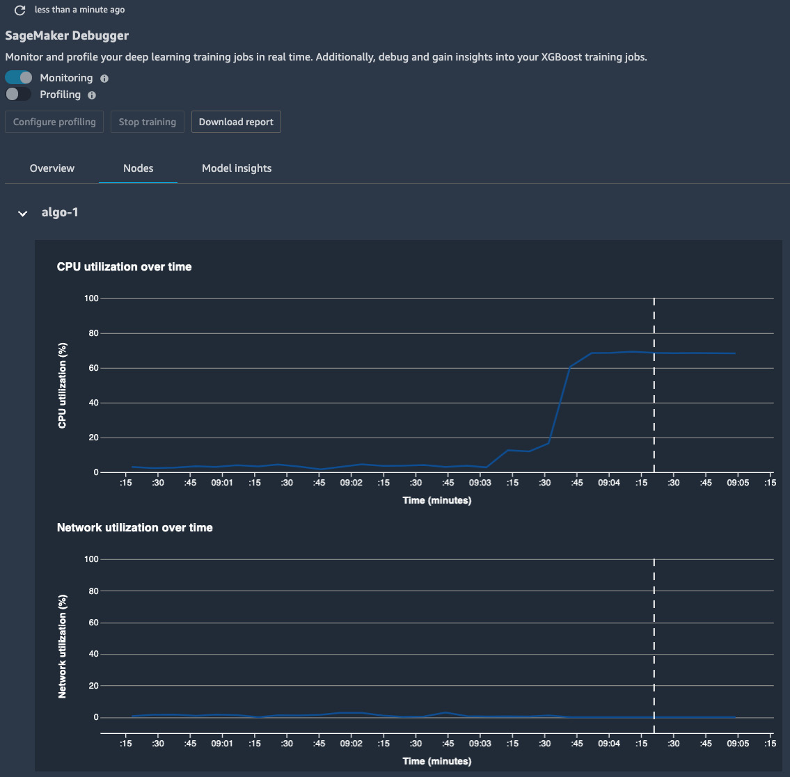
Figure 9.7 – The SageMaker Debugger insights dashboard showing the CPU and network utilization over the course of the training

In the Nodes tab, the mean utilization of the CPU, the network, the GPU, and the GPU memory are shown in the charts. You can narrow down the chart to a specific CPU or GPU to see whether there is any uneven utilization over the devices, as shown in Figure 9.8. From these charts, we can tell the following:

• The average CPU utilization peaked at around 60%, 3 minutes after the start of the job. This indicates that the training was taking place, and there was much activity on the CPU side to read in the data batches and feed into the GPU devices.
• The average GPU utilization over eight devices peaked at around 25%, also at 3 minutes after the start of the job. At the same time, there was around 5% of GPU memory used on average. This is considered low GPU utilization, potentially due to the small batch size compared to the now much larger compute capacity from an ml.p3.16xlarge instance.
• On the other hand, there was some network utilization in the first 3 minutes. This is the period when SageMaker's fully managed training downloaded the training data from the S3 bucket:

Figure 9.8 – The SageMaker Debugger insights dashboard showing the GPU utilization over the course of the training

At the bottom of the page, a heatmap of the CPU/GPU utilization in a holistic view is displayed. As an exercise, feel free to open the Debugger for the training job submitted at Getting-Started-with-Amazon-SageMaker-Studio/chapter06/02-tensorflow_sentiment_analysis.ipynb and compare the difference in the CPU/GPU utilization between single-device training and distributed training.

Next, we'll move on to learn how to lower the cost of training ML models in SageMaker Studio with fully managed spot training and how to create checkpointing for long-running jobs and spot jobs.

Managing long-running jobs with checkpointing and spot training

Training ML models at scale can be costly. Even with SageMaker's pay-as-you-go pricing model on the training instances, performing long-running deep learning training and using multiple expensive instances can add up quickly. SageMaker's fully managed spot training and checkpointing features allow us to manage and resume long-running jobs easily, helping us reduce costs up to 90% on training instances over on-demand instances.

SageMaker-managed Spot training uses the concept of spot instances from Amazon EC2. EC2 spot instances let you take advantage of any unused instance capacity in an AWS Region at a much lower cost compared to regular on-demand instances. The spot instances are cheaper but can be interrupted when there is a higher demand for instances from other users on AWS. SageMaker-managed spot training manages the use of spot instances, including safe interruption and timely resumption of your training when the spot instances are available again.

Along with the spot training feature, managed checkpointing is a key to managing your long-running job. Checkpoints in ML refer to intermediate ML models saved during training. Data scientists regularly create checkpoints and keep track of the best accuracy during the epochs. They compare accuracy against the best one during progression and use the checkpoint model that has the highest accuracy, rather than the model from the last epoch.

Data scientists can also resume and continue the training from any particular checkpoint if they want to fine-tune a model. As SageMaker trains a model on remote compute instances using containers, the checkpoints are saved in a local directory in the container. SageMaker automatically uploads the checkpoints from the local bucket to your S3 bucket. You can reuse the checkpoints in another training job easily by specifying their location in S3. In the context of SageMaker-managed spot training, you do not need to worry about uploading and downloading the checkpoint files in case there is any interruption and resumption of a training job. SageMaker handles it for us.

Let's run an example to see how things work. Open Getting-Started-with-Amazon-SageMaker-Studio/chapter09/03-spot_training_checkpointing.ipynb using the Python 3 (TensorFlow 2.3 Python 3.7 CPU Optimized) kernel and an ml.t3.medium instance. In this notebook, we will be reusing our TensorFlow model training for the IMDB review dataset from Chapter 5, Building and Training ML Models with SageMaker Studio IDE, and make some changes to the code to demonstrate how you can enable the checkpointing and managed spot training using SageMaker:

1. Run the first five cells to set up the SageMaker session, and prepare the dataset. If you ran the first chapter09/01-smdp_tensorflow_sentiment_analysis.ipynb notebook, the dataset should be available already.
2. The cell leading with %%writefile code/tensorflow_sentiment_with_checkpoint.py is where we will make changes to the TensorFlow/Keras code. First of all, we are adding a new --checkpoint_dir argument in the parse_args() function to assign a default /opt/ml/checkpoints location set by SageMaker.
3. In __name__ == '__main__', we will add a check to see whether checkpoint_dir exists locally in the container or not. If it does, list the directory to see whether there are any existing checkpoint files:

   if not os.listdir(args.checkpoint_dir):

       model = get_model(args)

       initial_epoch_number = 0

   else:    

       model, initial_epoch_number = load_model_from_checkpoints(args.checkpoint_dir)

If checkpoint_dir does not contain valid checkpoint files, it means that there is no prior training job and checkpoints attached to the container and that checkpoint_dir is newly created for brand-new model training. If it does contain files, it means that previous checkpoint files are plugged into this training job and should be used as a starting point of the training, implemented in the load_model_from_checkpoints() function.

4. Implement load_model_from_checkpoints() to list all the checkpoint files, ending with .h5, as this is how Keras saved the model, in a given directory and use regex from the re library to filter the epoch number in the filename. We can then identify the latest checkpoint to load and continue the training with such a model. We assume the epoch number ranges from 0 to 999 in the regular expression operation.
5. After the model is loaded, either a new one or from a checkpoint, implement a tf.keras.callbacks.ModelCheckpoint callback in Keras to save a model checkpoint to args.checkpoint_dir after every epoch.
6. When setting up the sagemaker.tensorflow.TensorFlow estimator, provide the following additional arguments to the estimator:
   1. use_spot_instances: A Boolean to elect to use SageMaker spot instances for training.
   2. max_wait: A required argument when use_spot_instances is True. This is a timeout in seconds waiting for the spot training job. After this timeout, the job will be stopped.
   3. checkpoint_s3_uri: The S3 bucket location to save the checkpoint files persistently. If you pass an S3 bucket location that already has checkpoint models and pass a higher epoch number, the script will pick up the latest checkpoint and resume training. For example, by providing checkpoint_s3_uri, which has checkpoints from a previous 50-epoch run and an epochs hyperparameter of 60, our script will resume the training from the fiftieth checkpoint and continue for another 10 epochs.
   4. max_run: The maximum runtime in seconds allowed for training. After this timeout, the job will be stopped. This value needs to be smaller than or equal to max_wait.

The following code snippet will construct an estimator to train a model with managed spot instances and checkpointing:

use_spot_instances = True

max_run = 3600

max_wait = 3600

checkpoint_suffix = str(uuid.uuid4())[:8]

checkpoint_s3_uri = f's3://{bucket}/{prefix}/checkpoint-{checkpoint_suffix}'

estimator = TensorFlow(use_spot_instances=use_spot_instances,

                       checkpoint_s3_uri=checkpoint_s3_uri,

                       max_run=max_run,

                       max_wait=max_wait,

                       ...)

7. The rest of the steps remain the same. We specify the hyperparameters, data input, and experiment configuration before we invoke .fit() to start the training job.
8. Wonder how much we save by using spot instances? From Experiments and trials in the left sidebar, we can bring up the AWS settings details of the trial, as shown in Figure 9.9, and see a 70% saving by simply using managed spot training instances:

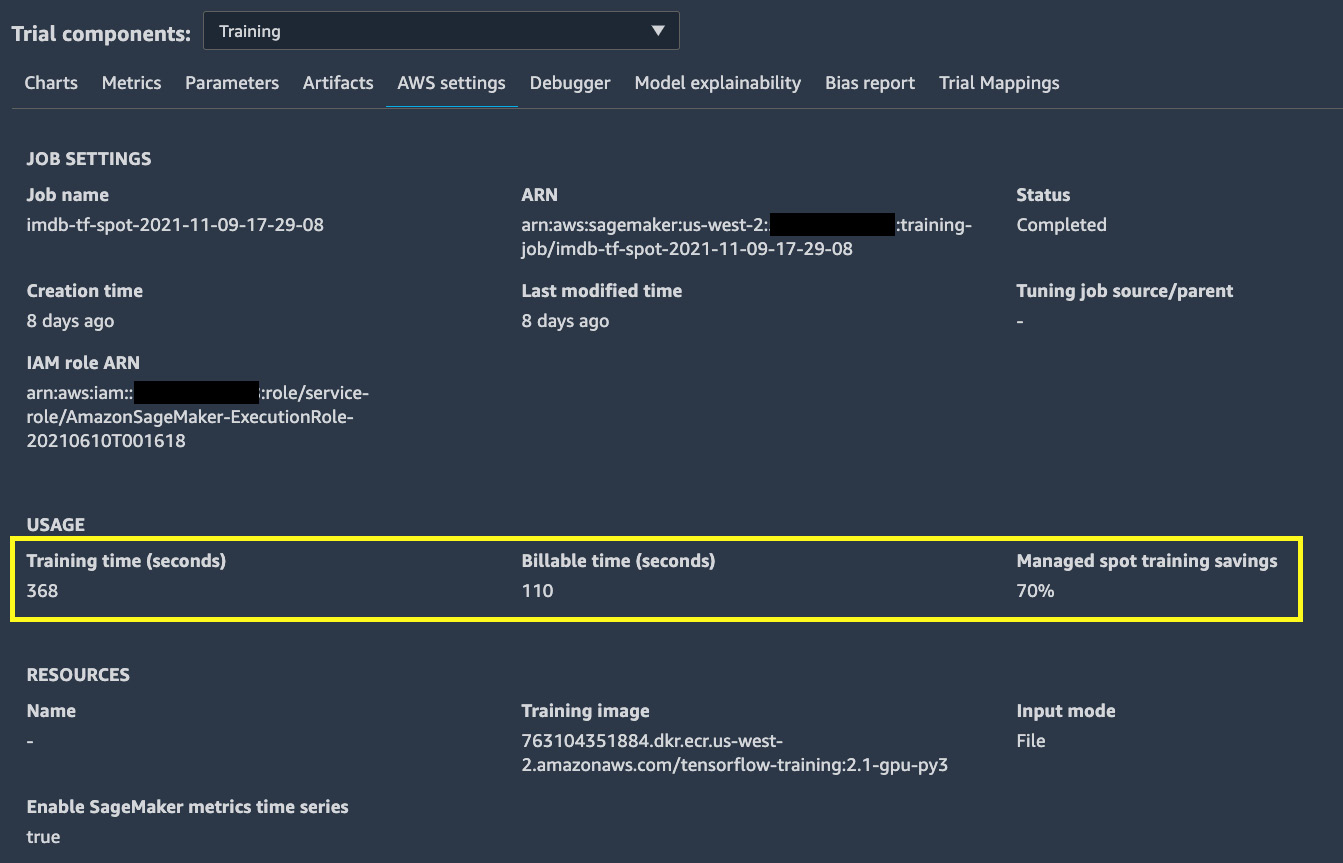
Figure 9.9 – A 70% saving using managed spot training, as seen in the trial details

A 70% saving is quite significant. This is especially beneficial to large-scale model training use cases that need expensive compute instances and have a long training time. Just four additional arguments to the estimator and some changes in the training script earn us a 70% saving.

Summary

In this chapter, we walked through how to train deep learning models using SageMaker distributed training libraries: data parallel and model parallel. We ran a TensorFlow example to show how you can modify a script to use SageMaker's distributed data parallel library with eight GPU devices, instead of one from what we learned previously. This enables us to increase the batch size and reduce the iterations needed to go over the entire dataset in an epoch, improving the model training runtime. We then showed how you can adapt SageMaker's distributed model parallel library to model training written in PyTorch. This enables us to train a much larger neural network model by partitioning the large model to all GPU devices. We further showed you how you can easily monitor the compute resource utilization in a training job using SageMaker Debugger and visualize the metrics in the SageMaker Debugger insights dashboard. Lastly, we explained how to adapt your training script to use the fully managed spot training and checkpointing to save costs when training models in SageMaker.

In the next chapter, we will be switching gear to learn how to monitor ML models in production. ML models in production taking unseen inference data may or may not produce quality predictions as expected from evaluations conducted prior to deployment. It is crucial in an ML life cycle to set up a monitoring strategy to ensure that your models are operating at a satisfactory level. SageMaker Studio has the functionality needed to help you set up model monitoring easily to monitor ML models in production. We will learn how to configure SageMaker Model Monitor and how to use it as part of our ML life cycle.