10

Working with Acceleration and Direction

In the previous chapter, we learned about the concepts of analog input and pulse-width modulation. We worked with analog devices such as potentiometers, photoresistors, and servo motors. We demonstrated their workings with the help of MicroPython examples in the previous chapter.

This chapter will explore the Micro:bit’s onboard components, such as an accelerometer and compass. We will design examples to understand the functioning of these onboard components. We will investigate the method of data storage in a local drive. We will also explore how to plot graphs for the data coming through an accelerometer. The methods involved in this chapter will be essential to handling complex hardware and data patterns. The following is the list of topics we will investigate and demonstrate in this chapter:

• Accelerometers
• Data logging and plotting
• Compasses
• Combining audio with a compass

Let’s explore them together.

Technical requirements

For this chapter, we will need the usual setup with a Micro:bit v2.

Accelerometer

An accelerometer is a device that measures the rate of change concerning the direction of force applied to it. It is a device that helps us to measure the vibrations, shock, tilt, and orientation in three dimensions. Now, the question may arise of how an accelerometer can carry out such measurements. Let us consider an example of palm-top devices. Based on the position of the user, the orientation of devices changes. If a user has a tablet PC and uses it horizontally to have a more comprehensive view, the auto-rotate option helps change the view to horizontal. Users don’t even need to make the change manually. This is because an accelerometer is working in real time and the change in orientation will be detected based on how the device is positioned. These features are also available in smartwatches (when you move your hand, the display will turn on), earpads (take them away from the ears and they automatically stop), and so on. Hence, accelerometers are now essential components of consumer electronics.

Let’s look at the position of the accelerometer on the Micro:bit:

Figure 10.1 – Position of the accelerometer on the Micro:bit board (courtesy: https://microbit.org/get-started/user-guide/overview/)

The accelerometer is attached to the Micro:bit board as an onboard component with a compass. Although accelerometers and other similar devices can be attached to hardware using the GPIO pins available, in the case of the Micro:bit, the availability of the onboard devices makes it easy to use and less complex for developers:

Figure 10.2 – Illustrating the accelerometer on a Micro:bit (courtesy: https://microbit-challenges.readthedocs.io/en/latest/tutorials/accelerometer.html)

As shown in Figure 10.2, on the tilt action in the X, Y, and Z directions, the displacement is calculated. The same can be viewed with the simple program demonstrated as follows: through the use of a built-in accelerometer.get_x() method, we get the acceleration value of the x axis, and the same can be done for the y and z axes too. The print() statement shows them in the shell window:

from microbit import *
while True:
    Tilt_x= accelerometer.get_x()
    print(“Tilt_x ", Tilt_x)
    sleep(1000)

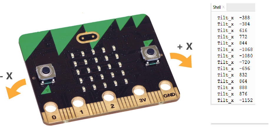
Figure 10.3 – Output of the program based on the tilt on the x axis

Figure 10.3 shows the output of the preceding program. As observed in the shell window, both positive and negative values are shown; the reason is also demonstrated in the Micro:bit diagram. Due to left and right movement on the x axis, both values will be visualized. If the accelerometer is tilted to the right, we will receive positive values, and negative values will be received when it is tilted to the left. The code, as mentioned earlier, can also be extended to obtain the value of the y and z axes.

In this section, we have explored the functionality of an accelerometer. We have also observed how to fetch the data from the accelerometer using the program. In the next section, we will see the data logging features and graph generation using an accelerometer.

Data logging

Figure 10.3 only shows the changes in the x axis data. Just one axis is insufficient for making effective decisions, such as fall detection, pitches, yaws, and rolls. We need to collect data from the x, y, and z axes. This data will make interpretation more accurate and reliable, as fall patterns can’t be analyzed just from one axis. Hence, it is essential to have data stored in a file so it can be used for analysis. Data logging is a method of storing the data coming from sensors, actuators, or any subsystems to keep a record, which will further help decision-making and monitoring. Data visualization is equally essential; it is easier to observe the significant changes via graphs and figures.

In the following program, the movement of the Micro:bit board is recorded with the help of an accelerometer. Based on the tilt, we are displaying the image on an LED array display:

from microbit import *
while True:
    sleep(120)
    print(accelerometer.get_values())
    movement = accelerometer.current_gesture()
    if movement == “shake”:
        display.show(Image.ANGRY)
    else:
        display.show(Image.HAPPY) 

In the preceding program, accelerometer.get_values() fetches the values for the x, y, and z axes. Based on the input values, the shake motion is being executed; this means that when the user shakes the Micro:bit board, it will display an angry gesture, and the happy gesture will be displayed in a normal state.

For this particular program, we are using the Mu editor. The advantage of the Mu editor is that it can show the plot graph and the accelerometer’s real-time values:

Figure 10.4 – Illustrating the functionality of the Mu editor

As shown in Figure 10.4, using the Mu editor, we can check the code functionality by clicking on the Check icon. Apart from that, the code can directly be flashed to the Micro:bit using the Flash icon. By clicking on REPL, it will show the real-time values of the accelerometer. The graph can be plotted using the Plotter icon shown on the toolbar. The three signals in the Plotter window represent the x, y, and z values from the accelerometer. The signals in the graph represent x, y, and z coordinates, ranging from positive and negative values based on the motion detected in real time. The data log is also available in the local repository.

As shown in Figure 10.5, to track the data location, we need to go to the Mu editor’s local repository, that is, mu_code:

Figure 10.5 – Data log saved in the data_capture folder of mu_code

Inside the folder, we need to find the data_capture folder, as shown in step 2 of Figure 10.5. Once we get inside the folder, the Excel file can be seen, as in Figure 10.6:

Figure 10.6 – Data saved as an Excel file and the values coming from the accelerometer

The Excel files are stored with a date and time stamp, so it would be easy for us to trace the data logs we are looking for. For example, in the 20220810-110618 filename, 20220810 represents the date in the YYYY-MM-DD format, and 110618 represents the time in the HH-MM-SS format.

In the preceding program, we have seen the usefulness of the Mu editor and have also gone through the data folders and files. In the next section, we will explore the compass and its application.

Compasses

Also known as a magnetometer, a compass measures the magnetic fields and is also an essential instrument for drones and aircraft to check the direction for navigation-related applications. In Micro:bit, as shown in Figure 10.7, the compass is mounted on the board. The functionality of the compass is such that it finds North at 0 degrees and 315 degrees as North West:

Figure 10.7 – Micro:bit with a compass, illustrating directions with degrees (courtesy: https://microbit.org/projects/make-it-code-it/compass-north/)

From the figure, we can observe that South is at 180 degrees, East is at 90 degrees, and West is at 270 degrees. Hence, now, it is easier to track the direction using the compass, but first, we need to calibrate the compass. The compass.calibrate() function is used to perform the calibration:

from microbit import *
compass.calibrate()

In this process, the Micro:bit display panel will display the Tilt to fill screen message, scrolled onscreen, to rotate the board. Once it stops, for calibration, we need to tilt the Micro:bit board in all directions so that the LEDs on the Micro:bit board will be turned on. Please make sure that the program runs till all the LEDs are turned on, as shown in Figure 10.8:

Figure 10.8 – Display when the calibration LEDs are turned on

Once the calibration process is complete, a smiling face will appear for a short amount of time as shown in Figure 10.9:

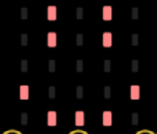
Figure 10.9 – After calibration, a smiley face appears, meaning the calibration is successful

After this, the screen will go blank, which signifies the process is finished, and the board is ready to track the direction in degrees through the heading:

from microbit import *
while True:
    print(compass.heading())
    sleep(300)

In the preceding program, the heading rotation will be displayed. The values will be given as 0 to 360 angles in degrees using compass.heading():

Figure 10.10 – Display of the heading values from 0 to 359

Figure 10.10 shows the outcomes of the preceding program. 359 and 0 indicate North, 198 is close to South, and so on.

Similar to calibration and heading, we can also calculate the magnitude of the magnetic field around the Micro:bit:

from microbit import *
while True:
    print(compass.get_field_strength())
    sleep(300)

In the preceding code, compass.get_field_strength() indicates the values in nanotesla (nT):

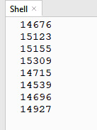
Figure 10.11 – Display of the output values of the magnitude of the magnetic field in nT

As indicated in Figure 10.11, the outputs can vary by variation in magnetic field strength.

Similar to observing magnetic field strength, we can also visualize the x, y, and z coordinate values of the compass. It can be done using the inbuilt compass.get_ functions as seen in the following program:

from microbit import *
while True:
    degrees=compass.heading()
    magnitude= compass.get_field_strength()
    x_values = compass.get_x()
    y_values = compass.get_y()
    z_values = compass.get_z()
    print(‘degrees:{} magnitude:{} x_values:{} y_values:{} z_values{}' .format(degrees, magnitude, x_values, y_values, z_values))
    sleep(300)

In the program, we have assigned five variables as degrees for the heading, magnitude for the magnetic field strength, and x_values, y_values, and z_values for retrieving the values of the x, y, and z coordinates. compass.get_y() will provide the data for the y coordinates of the compass and the values for the x and z coordinates will also be retrieved using compass.get_x() and compass.get_z(). At the end of the code, the print will show the outcomes on the shell window, as shown in Figure 10.11:

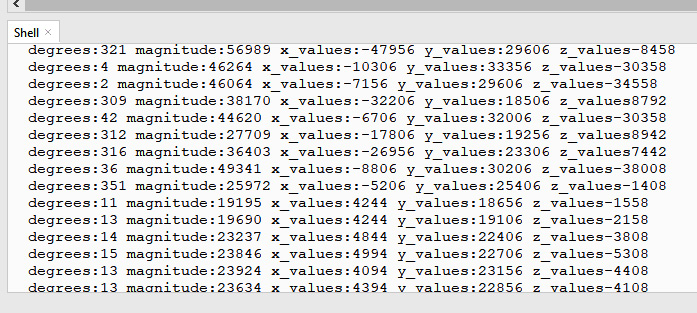
Figure 10.12 – Illustration of headings in degrees, the magnitude, and the x, y, and z coordinate values in the shell window

In this section, we have gone through the basic features of a compass and its application. We have also observed with the help of a program that it can display headings and field strength for magnetic fields nearby. We have also been able to visualize the values from the compass, such as degrees, magnitudes, and x, y, and z axes values.

Audio and compass

This section will try to integrate the speech library and compass to assist with the direction information. The speech library will convert the heading into audio, and we have already observed the working of the heading function in the previous example. The code will be as follows:

from microbit import *
import speech
import music
while True:
    direction = compass.heading()
    print(direction)
    if direction < 35 :
        speech.say(“North”)
        display.scroll(“N”)
        music.play(“E8:4”)
    elif direction == 90: 
        speech.say(“East”)
        display.scroll(“E”)
        music.play(“D8:4”)
    elif direction == 180: 
        speech.say(“South”)
        display.scroll(“S”)
        music.play(“C8:2”)
    elif direction == 270: 
        speech.say(“West”)
        display.scroll(“W”)
        music.play(“B8:2”)

Two libraries, music and speech, are imported into the preceding program. The music library will be used for playing the musical notes, whereas the sound library will play the speech. In the program, a variable name is initialized as a direction, which will collect the values for the heading information based on the heading data; North, South, East, and West directions will be recognized. After executing the program, when a user rotates the Micro:bit board, a specific tone and speech will be played once pointed in a specific direction.

Summary

In this chapter, we have explored the onboard components of the Micro:bit board, such as an accelerometer and a compass. Both are complex components with usage in real-life applications such as fall detection, shock analysis, and navigation. We have also explored data logging techniques using an accelerometer. We have also gone through compass programming using various methods. We also explored inbuilt functions and methods, such as accelerometer.get_values, compass. calibrate(), compass.heading(), and compass.get_field_strength().

In the next chapter, we will explore NeoPixel programming and interfacing with a MAX7219-based 8-digit Seven Segment display board.

Further reading

We can find more information about the accelerometer and compass in a Micro:bit implementation of MicroPython at https://microbit-micropython.readthedocs.io/en/v2-docs/accelerometer.html and https://microbit-micropython.readthedocs.io/en/v2-docs/compass.html.