
6
Single Flow Crossing Several Servers
The previous chapter focused on the analysis of a single flow crossing a single server. Before handling more complex topologies in Part 3, we consider in this chapter the fundamental case of one flow of data crossing a sequence of servers. This is a typical network in the network calculus literature for several reasons. First, it can be easily solved using (min,plus) operations: the main result of this chapter is the correspondence between concatenation of servers and (min,plus) convolution. Second, we will see in the next chapters that one solution to analyze more general topologies is to individualize the service curves, and the final step of the analysis is to compute the performance of one flow crossing a sequence of servers.
The algebraic formulation enables us to compute performance guarantees for the flow, such as delays. Intuitively, worst-case delay of a bit of data crossing a sequence of servers is smaller than the sum of the worst-case delays for each server computed with the results of Chapter 5. This is known as the pay burst only once phenomenon. This will be discussed in section 6.1.
Another type of network involving one flow of data is for control purposes. This can be performed by adding a server in front of a network in order to gain some control over the departure process of this added server, i.e. the arrival process in the rest of the network. Another solution is to add a feedback loop that regulates the arrivals in a part of the network. This will be the topic of section 6.2.
Finally, section 6.3 presents some classical use cases explaining in detail the modeling of flows and servers in the network calculus framework.
6.1. Servers in tandem
In this section, we consider one flow crossing a sequence of servers, or a tandem. We assume that each server is crossed only once. Such a network is depicted in Figure 6.1. In this example, server Si has cumulative arrival process Ai and cumulative departure process Ai+1, which means that the departure process of a server is the arrival process of the next. As no data is created nor lost in a server, each bit of data crosses each server along the same path. This is what is meant by the denomination flow of data, or flow for short.
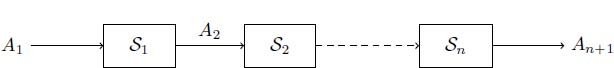
Figure 6.1. A single flow crossing servers in tandem
In this section, we first define the concatenation of servers in section 6.1.1. This will enable us to state the correspondence between the concatenation of servers and the (min,plus) convolution. This will be the basis for the illustration of the pay burst only once phenomenon in section 6.1.2. Finally, we will discuss the case of the composition of strict service curves in section 6.1.3.
6.1.1. Concatenation and service convolution
In this section, we focus on the small network, composed of two servers, of Figure 6.2. The results are here stated for two servers in sequence, but can easily be generalized using the associativity of the (min,plus) convolution.

Figure 6.2. Concatenation of servers. For a color version of this figure, see www.iste.co.uk/bouillard/calculus.zip
DEFINITION 6.1 (Concatenation of servers).– Let ![]() , the concatenation of S1 and S2 is
, the concatenation of S1 and S2 is
If ![]() , we denote
, we denote ![]() and
and ![]() .
.
PROPOSITION 6.1.– If S1 and S2 are two servers, then so is ![]() .
.
PROOF.– Servers S1 and S2 are two left-total binary relations, so it is also the case for ![]() .Moreover, for all
.Moreover, for all ![]() , there exists B ∈ C such that
, there exists B ∈ C such that ![]() and
and ![]() , and 0 ≤ C ≤ B ≤ A. Thus, 0 ≤ C ≤ A, and
, and 0 ≤ C ≤ B ≤ A. Thus, 0 ≤ C ≤ A, and ![]() is a server.
is a server.
□
In order to conform to the order in which the servers are crossed by the flow, the concatenation of servers S1 and S2 can also be denoted as S1 ; S2. In addition, since the composition is associative, the definition of the concatenation can be straightforwardly generalized to a sequence of n servers.
We can now state the central result of this section.
THEOREM 6.1 (Concatenation of servers in a convolution).– A flow crossing two servers respectively offering min-plus service curves β1 and β2 is globally offered a min-plus service curve β1 ∗ β2. In other words,
The same holds for maximal service curves:
PROOF.– Denote S1 = Smp(β1) and S2 = Smp(β2). For all ![]() , there exists B ∈ C such that (A, B) ∈ S1 and (B, C) ∈ S2. Thus, A ≥ C ≥ B ∗ β2 ≥ (A ∗ β1) ∗ β2 = A ∗ (β1 ∗ β2), using the isotony and the associativity of the (min,plus) convolution. Thus, (A, C) ∈ Smp (β1 ∗ β2).
, there exists B ∈ C such that (A, B) ∈ S1 and (B, C) ∈ S2. Thus, A ≥ C ≥ B ∗ β2 ≥ (A ∗ β1) ∗ β2 = A ∗ (β1 ∗ β2), using the isotony and the associativity of the (min,plus) convolution. Thus, (A, C) ∈ Smp (β1 ∗ β2).
Similarly, if now S1 = Smax(β1) and S2 = Smax(β2), then (with the same notations) C ≤ B ∗ β2 ≤ (A ∗β1) ∗ β2, so (A, C) ∈ Smax(β1 ∗ β2).
□
Remark that the (min,plus) convolution is a commutative operator, whereas the composition is not. This means that the convolution does not exactly model the composition. Indeed, the inclusion may be strict: let β1 = δ3 and β2 = λ1, ![]() and
and ![]() . It is easy to check that A ≥ C ≥ A ∗ β1 ∗ β2. Now, given A and C, the minimal admissible departure process from the first server is B = max(C, A ∗ β1). However,
. It is easy to check that A ≥ C ≥ A ∗ β1 ∗ β2. Now, given A and C, the minimal admissible departure process from the first server is B = max(C, A ∗ β1). However, ![]() . Those functions are depicted in Figure 6.3. As the convolution is an isotone operator, we can conclude that there does not exist B ∈ C, such that (A, B) ∈ Smp(β1) and (B, C) ∈ Smp(β2).
. Those functions are depicted in Figure 6.3. As the convolution is an isotone operator, we can conclude that there does not exist B ∈ C, such that (A, B) ∈ Smp(β1) and (B, C) ∈ Smp(β2).
It will be shown in section 6.1.3 that the concatenation property does not hold for strict service curves.
6.1.2. The pay burst only once phenomenon
To illustrate the pay burst only once phenomenon, let us focus on the example of two servers of Figure 6.2 and the cumulative processes depicted in Figure 6.4. Packets of unit size cross the servers. In the first server, d(A, B) = 4, which is obtained for the second packet, and in the second server, d(B, C) = 4, which is obtained for the first and third packets. However, globally, we have d(A, C) = 7 < 8 = d(A, B) + d(B, C).
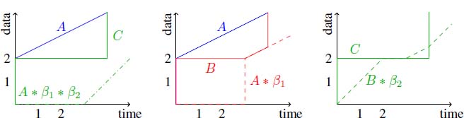
Figure 6.3.  . Left: A ≥ C ≥ A ∗ β1 ∗ β2; center: A ≥ B ≥ max(C,A ∗ β1);
right: C and B ∗ β2 cannot be compared. For a color version
of this figure, see www.iste.co.uk/bouillard/calculus.zip
. Left: A ≥ C ≥ A ∗ β1 ∗ β2; center: A ≥ B ≥ max(C,A ∗ β1);
right: C and B ∗ β2 cannot be compared. For a color version
of this figure, see www.iste.co.uk/bouillard/calculus.zip

Figure 6.4. Pay burst only once phenomenon. For a color version of this figure, see www.iste.co.uk/bouillard/calculus.zip
More generally, with the results of Chapter 5 and the previous section, there are two ways of computing upper bounds on the delay in a sequence of servers.
If we do not use this concatenation property, a delay bound can be computed in the following way:
- 1) compute d1 the delay for the first server
 ;
; - 2) compute
 ;
; - 3) compute d2 the delay for the first server
 ;
; - 4) a worst-case delay bound is d1 + d2.
When using Theorem 6.1, a delay bound can be computed as
which always gives better bounds, as explained below.
Intuitively, with the first method, a burst will induce a delay in each server. However, if the first server introduces a delay, it also smooths the arrivals to the second server. Thus, if a burst is delayed at the first server, when the last bit of data of this burst arrives in the second server, the rest of the burst has already started being processed by the second server. As a result, the last bit of data does not have to pay again the delay induced by the burst, hence the name. Conversely, if the first server forwards the burst as it is, it does not introduce any delay.
More precisely, if ![]() , we have
, we have ![]()
![]() . If S1 = Smp(β1) and S2 = Smp(β2), and the flow is α-constrained, then A = α, B = min(β1, α), C = min(α, β1 ∗ β2) is an admissible trajectory for the tandem network that satisfies
. If S1 = Smp(β1) and S2 = Smp(β2), and the flow is α-constrained, then A = α, B = min(β1, α), C = min(α, β1 ∗ β2) is an admissible trajectory for the tandem network that satisfies ![]() . But,
. But,
As a result,
or equivalent d ≤ d1 + d2.
To quantify the difference, if the services are rate-latency ![]() and the arrival curve token-bucket
and the arrival curve token-bucket ![]() , with
, with ![]() , using Propositions 3.5 and 3.7, we have
, using Propositions 3.5 and 3.7, we have ![]()
![]() , i.e. the sum of individual delays leads to the delay bound
, i.e. the sum of individual delays leads to the delay bound

The application of Theorem 6.1 states that the sequence of servers offers the
service ![]() (see Proposition 3.4), leading to a delay
(see Proposition 3.4), leading to a delay
Note that ![]() . Computing the delay using the concatenation of servers, only one term related to the burst appears,
. Computing the delay using the concatenation of servers, only one term related to the burst appears, ![]() , whereas computing per server delay adds two other terms,
, whereas computing per server delay adds two other terms, ![]() and
and ![]() , that depend on the order of the servers.
, that depend on the order of the servers.
6.1.3. Composition of strict service curves
WARNING.– It is not true in general that a system composed of two strict service curves in tandem offers a strict service curve, as shown by the following proposition.
PROPOSITION 6.2.– Let β1 and β2 be two functions such that there exist T1, T2 > 0 with β1(T1) = 0 and β2(T2)=0. Then, ![]() such that
such that ![]()
![]() .
.
PROOF.– As ![]() , it suffices to show the result for
, it suffices to show the result for ![]() .
.
Consider an arrival cumulative process A defined the following way: fix b > 0 and ![]() , then
, then ![]() ,
,

Note that A(t) is constrained by ![]() .
.
Now let us compute B a possible departure process from the first server, and C a possible departure process from the second server.
Since T > T1, it is possible to choose ![]() , and since T > T2, it is possible to choose
, and since T > T2, it is possible to choose ![]()
![]() . The trajectory is depicted in Figure 6.5.
. The trajectory is depicted in Figure 6.5.

Figure 6.5. No strict service curve for two servers in tandem. For a color version of this figure, see www.iste.co.uk/bouillard/calculus.zip
From this figure, we see that the system is always backlogged. Indeed, ![]() ,
, ![]() since by definition, A(t) > A
since by definition, A(t) > A ![]() .
.
Thus, if β were a strict service curve for the system, it would hold that β ≤ C ≤ A ≤ ![]() . When T is fixed, this should hold for all b > 0. Then, the only possible strict service curve is β = 0.
. When T is fixed, this should hold for all b > 0. Then, the only possible strict service curve is β = 0.
□
However, when β1 = λR1 and ![]()
![]() . Indeed, a backlogged period (s, t] can be divided into intervals where the second server is backlogged and intervals where it is not (and where server 1 is therefore backlogged). Let
. Indeed, a backlogged period (s, t] can be divided into intervals where the second server is backlogged and intervals where it is not (and where server 1 is therefore backlogged). Let ![]() be the total length where the second server is backlogged and
be the total length where the second server is backlogged and ![]() that where it is not. We have
that where it is not. We have ![]() . When server 2 is backlogged, the departure rate is at least R2. When it is not, the departure rate is at least R1: server 1 is backlogged but not server 2, so the service of server 2 follows that of server 1. The service offered is then at least
. When server 2 is backlogged, the departure rate is at least R2. When it is not, the departure rate is at least R1: server 1 is backlogged but not server 2, so the service of server 2 follows that of server 1. The service offered is then at least ![]() .
.
The loss of the strict character of the service curves with the concatenation raises issues that will be explained in section 9.3.
6.2. Control design
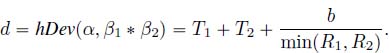
In Chapter 5, tools were given to compute and analyze performances of a server, especially concerning its delay and memory usage through deviations hDev and vDev. In this section, we address the problem of control. Control is useful to guarantee the behavior of a system. For example, we may want to ensure that the number of packets, or the delay of packets, in a system never exceeds some fixed value.
In this section, we model a system by a server and focus on two types of control, which are respectively studied in sections 6.2.1 and 6.2.2:
- – tandem control: a filter is added in front of the server;
- – feedback control: a feedback loop is added to the server.
The entire network obtained with the server and the control element is called the controlled network.
6.2.1. Tandem control
The tandem control design has a direct influence on the arrival flow of the server since the filter is linked to its input as illustrated in Figure 6.6. The process A' is the arrival cumulative function of the server (after the filter), whereas A is the arrival cumulative function of the filter. The service curve of the server is β and the service curve of the filter is βc.
The question is: given the behavior of the server on the right, modeled by a minimum min-plus service curve β, and given a reference target behavior modeled by a service curve βref or a performance requirement, how to design the server on the left, i.e. how to choose βc?

Figure 6.6. Tandem control design
When the left server is modeled by a min-plus service curve βc, the controlled network is guaranteed the service curve βc ∗ β from Theorem 6.1. It is not always possible to find βc such that βc ∗ β = βref. To guarantee the behavior, we want to ensure that βc ∗ β ≥ βref.
PROPOSITION 6.3.– Let βref be the min-plus service curve the controlled network has to reach. The smallest service curve βc, such that βc ∗ β ≥ βref, is
PROOF.– This is a direct application of Proposition 2.7.
□
Control by a greedy shaper. The tandem control might be too permissive. Indeed, it adds undeterminism to the system, as necessarily, βref ≤ β. It might thus be more useful to use a controller that reduces the undeterminism of the system. One way is to use greedy shapers instead. In this type of system, we want a guarantee to be satisfied on the server offering service curve β, and not on the controlled system anymore. A shaper will then give a guarantee on the arrival curve of A'.
The objective is then to find the arrival curve α for A' that ensures some guarantees for the next server. The controller will then be an α-greedy shaper. The guarantees are classically upper bounds on the delay or on the backlog. The largest curve to choose is given by the following propositions.
PROPOSITION 6.4.– Let ![]() be the service curve of a server S and
be the service curve of a server S and ![]() be a fixed maximal delay. If
be a fixed maximal delay. If ![]() , then
, then ![]() . In other words, the delay in server S never exceeds
. In other words, the delay in server S never exceeds ![]() when it is crossed by an α-constrained arrival process. Moreover,
when it is crossed by an α-constrained arrival process. Moreover, ![]() is the largest sub-additive function that has this property.
is the largest sub-additive function that has this property.
PROOF.– By Proposition 5.12, for all ![]() .By Proposition 3.2,
.By Proposition 3.2, ![]() ,so
,so ![]() . To conclude the first part of the proof, if α is an arrival curve for a process, so is α∗, which is sub-additive.
. To conclude the first part of the proof, if α is an arrival curve for a process, so is α∗, which is sub-additive.
Now, consider a sub-additive function α such that ![]() for some t; thus,
for some t; thus, ![]() . As α is sub-additive,
. As α is sub-additive, ![]() , which proves the optimality of
, which proves the optimality of ![]() .
.
□
PROPOSITION 6.5.– Let ![]() be the service curve of a server S and b be a fixed maximal backlog. If
be the service curve of a server S and b be a fixed maximal backlog. If ![]() , then
, then ![]() . In other words, the backlog in server S never exceeds b when it is crossed by an α-constrained arrival process. Moreover, (β + b)∗ is the largest sub-additive function that has this property.
. In other words, the backlog in server S never exceeds b when it is crossed by an α-constrained arrival process. Moreover, (β + b)∗ is the largest sub-additive function that has this property.
PROOF.– From Proposition 5.12, for all ![]() . But
. But ![]() , so
, so ![]() .
.
Now, consider a sub-additive function α such that there exists t with ![]() . Thus,
. Thus, ![]() . As α is sub-additive,
. As α is sub-additive, ![]() , which proves the optimality of
, which proves the optimality of ![]() .
.
□
These propositions can be used to compute an arrival curve in order to respect a maximal delay or backlog, assuming that the minimum service curve of the server is known. This largest arrival curve is said to be optimal because it is the less restrictive one where the given delay is not exceeded.
6.2.2. Feedback control
The feedback control is a design where the arrival cumulative function A is affected by the departure function D as illustrated in Figure 6.7. The ![]() symbol corresponds to synchronization: the arrival function A' (arrival at the server) is synchronized between A and
symbol corresponds to synchronization: the arrival function A' (arrival at the server) is synchronized between A and ![]() .
.

Figure 6.7. Feedback control design
The closed-loop network in this feedback design obeys the equations:

As a result, ![]() , and from Theorem 2.3,
, and from Theorem 2.3, ![]() and
and
Then, the service curve of the closed-loop network is β ∗ (βc ∗ β)∗.
Here again, we call βref a service curve for the controlled network, and we want to compute a controller (i.e. a service curve βc) such that the controlled system is guaranteeda βref min-plus service curve: we want to ensure that β ∗ (βc∗ β)∗ ≥ βref.
PROPOSITION 6.6.– Let βref be the min-plus service curve that the controlled network has to reach. The smallest service curve βc, such that β ∗ (βc∗ β)∗ ≥ βref, must satisfy
PROOF.– We have the equivalences

The inequalities use Proposition 2.7 and the associativity of the convolution.
□
Window flow control. The so-called window flow control mechanism (see [AGR 99, CHA 00, LEB 01]) is the use of the feedback control design, where we want to ensure that the backlog never exceeds some value ![]() for all
for all ![]() ,
, ![]() . This is the feedback control when
. This is the feedback control when ![]() , with
, with ![]() for t > 0 and
for t > 0 and ![]() . This configuration is shown in Figure 6.8 with β the service curve of the server.
. This configuration is shown in Figure 6.8 with β the service curve of the server.

Figure 6.8. Window flow control design
PROPOSITION 6.7.– Consider the network of Figure 6.8. The controlled network has minimal min-plus service curve ![]() .
.
PROOF.– Replace βc with ![]() in equation [6.3], so
in equation [6.3], so ![]() .
.
□
From a flow regulation point of view, it can be interesting to keep identical the service β provided by the server without degradation, although this server is enclosed in this closed-loop design. This is given by the following proposition.
PROPOSITION 6.8.– If ![]() , then
, then ![]() .
.
Note that if βwfc ≥ β, then βwfc = β. Indeed, as ![]()
![]() To prove the proposition, we need the following lemma.
To prove the proposition, we need the following lemma.
LEMMA 6.1.– If ![]() , then for all
, then for all ![]() .
.
PROOF.– We first compute, using Proposition 6.6, the best controller with βref = β: we must find βc such that ![]() . First
. First ![]() so the case n = 0 always holds. Second, from the case n = 1, we must take
so the case n = 0 always holds. Second, from the case n = 1, we must take ![]() . Let us show that, if
. Let us show that, if ![]() , then
, then ![]() for all n > 1.
for all n > 1.
We proceed by induction. This is true for n = 1 by hypothesis. Assume that it is true for n − 1, and show it for n. We have

where we used in the second line the fact that ![]() .
.
□
PROOF OF PROPOSITION 6.8.– We apply Lemma 6.1 to ![]() satisfying
satisfying ![]()
![]() .
.
□
In a window flow control configuration, a difference can be made between the data flow (from the source to the destination) and the acknowledgments flow (from the destination to the source). This configuration is illustrated in Figure 6.9 with β for the service curve of the data flow and βack for the service curve of the acknowledgment flow.
The main interest of this distinction is that the acknowledgments require considerably less bandwidth than the data itself (see [AGR 99]). Thus, the computation of the window size will have the benefit of this profit of bandwidth.
The equations of this window flow controlled network are


Figure 6.9. Window flow control design with acknowledgments
Thus, in the same way as we obtained equation [6.3], the service curve of the window flow controlled network is
PROPOSITION 6.9.– If ![]() , then βwfc-ack ≥ β.
, then βwfc-ack ≥ β.
PROOF.– We apply Lemma 6.1 with the service curve βc of the form ![]() . The service curve βc must satisfy
. The service curve βc must satisfy ![]() which is equivalent to
which is equivalent to ![]()
![]() .
.
□
Finally, the last result can be extended to the cases where maximal service curves are known. We denote the maximal service curves βM for the data and ![]() for the acknowledgments. In that case, it is possible to compute the window size that will not damage the service provided. This situation is illustrated in Figure 6.10.
for the acknowledgments. In that case, it is possible to compute the window size that will not damage the service provided. This situation is illustrated in Figure 6.10.

Figure 6.10. Window flow control design: minimal and maximal service curves
We of course assume that βM ≥ β and ![]() .The equations of the network become
.The equations of the network become

Similar to equation [6.4], we obtain that the global service curve of the system is at least ![]() . Concerning the upper bound, a simple induction shows that
. Concerning the upper bound, a simple induction shows that

As ![]() and
and ![]() for any β and βM, it remains to compute the value of
for any β and βM, it remains to compute the value of ![]() such that
such that ![]() and
and![]() .
.
From Proposition 6.9, this is obtained for
6.3. Essential use cases
Chapter 5 presented the basics of network calculus and the first section of this chapter was devoted to the analysis of a sequence of servers. In this section, we focus on the modeling aspect of network calculus, and show how it can be used in practice.
Our first interest will be on modeling servers, and then on modeling flows of data. Note that as we still deal with only one flow crossing servers, we will not mention service policies, which will be the topic of Chapters 7 and 8. We do not give the details of the computations, which have already been tackled in section 3.1.
6.3.1. Essential services curves
The basic models for servers are: the constant rate server, the delay guarantee, the jitter and the rate-latency server. They rely on the usual functions presented in section 3.1. These basic blocks are sufficient to model a wire with fixed capacity, or to abstract a system whose details are unknown.
In this section, we denote by A the cumulative arrival function and D the cumulative departure function of the server that we model.
6.3.1.1. Guaranteed or constant-rate servers
The constant-rate server was used to introduce the notion of service curve in section 1.2. We first reintroduce it in view of the formalization presented in Chapter 5.
A guaranteed-rate server offers a minimum throughput. It can, for example, be a wire offering at least a 100 Mb/s throughput. If this system is perfect, i.e. whenever there is some backlog, the departure throughput is at least of 100 Mb/s. More formally, on any backlogged period (s, t],
Then, such a system offers a strict service curve λR, with R = 108b/s. Since a strict service curve is also a min-plus service curve, as stated in Proposition 5.7, the server also offers a min-plus service curve λR.
A constant-rate server is a server that serves data exactly at rate R for some R. As a result, it is also a maximal service curve: ![]()
![]() . Consequently, from Proposition 5.11, a constant-rate server with rate R is also a λR-greedy shaper.
. Consequently, from Proposition 5.11, a constant-rate server with rate R is also a λR-greedy shaper.
The constant-rate server is an idealized case. It sometimes happens that the system has a clock drift. For example, if there is a 1% drift of the clock, then the 100 Mb/s link might have a service rate between 99 Mb/s and 101 Mb/s, leading to a strict service curve λ99.106 and a maximal service curve λ101.106.
6.3.1.2. Delay and jitter guarantees
In the previous section, the behavior of the constant-rate server was precisely known. It is often the case that only partial information about the server is available, and service curves then have to be derived from this knowledge. This is particularly the case when information about delays is known.
If the transmission delay of each bit of data is at least dm and at most dM, then we have the inequalities ![]() ,
,
In other words, ![]() . The behavior of the server can then be abstracted by pure delay service curves (a min-plus service curve
. The behavior of the server can then be abstracted by pure delay service curves (a min-plus service curve ![]() and a maximum service curve
and a maximum service curve ![]() ).
).
From Theorem 5.3, if α is an arrival curve for A, an arrival curve of D is ![]() . The latter equality comes from Proposition 3.2. The quantity dM − dm is called the jitter.
. The latter equality comes from Proposition 3.2. The quantity dM − dm is called the jitter.
In particular, if the departure function is exactly shifted by d (i.e. dm = dM = d), then the output departure process is constrained by α. Note that as δd is not subadditive, Proposition 5.11 cannot be applied, and the server is not a δd-greedy shaper.
Moreover, remark that guaranteeing a delay cannot be modeled by a strict service curve of type δd. Indeed, if a server offers a strict service curve δd, any backlogged period is bounded by d. Indeed, if t − s > d, ![]() , so (s, t] cannot be a backlogged period, whereas having a guaranteed delay does not impose any constraint on the length of a backlogged period.
, so (s, t] cannot be a backlogged period, whereas having a guaranteed delay does not impose any constraint on the length of a backlogged period.
More formally, we can state the following theorem: it is possible to deduce pure delay min-plus and maximal service curves from the delay guarantees of the server.
THEOREM 6.2 (Server as a jitter).– Let S be a server and A be an arrival cumulative process. If the delay in the server for every bit of data is always between dm and dM, then S offers to A a min-plus service curve δ dM and a maximal service curve δdm.
More precisely, for all (A, D) ∈ S,
This results can be used in two ways: first, it can be difficult to build a tight service curve that is associated with a server (because of its service policy, for example), whereas the guaranteed delay can be evaluated using some specific methods; second, although a service curve β can be identified, the computation of the deconvolution with β can be algorithmically complex, whereas from Proposition 3.2, the deconvolution by a pure-delay function is just a time-shift.
PROOF.– First, assume that ![]() and recall that
and recall that ![]()
![]() . Then, for all
. Then, for all ![]() . As D is left-continuous, letting d grow to dm leads to
. As D is left-continuous, letting d grow to dm leads to ![]() .
.
For the second statement, we proceed by contraposition. Assume that there exists t such that ![]() . Necessarily, t > dM, as A(0) = D(0) = 0. From the definition of the (min,plus) convolution, for all s ≤ t, and in particular, D(t) < A(t − dM). With u = t − dM, we reformulate D(u + dM) < A(u). But from the alternative definition of the horizontal deviation,
. Necessarily, t > dM, as A(0) = D(0) = 0. From the definition of the (min,plus) convolution, for all s ≤ t, and in particular, D(t) < A(t − dM). With u = t − dM, we reformulate D(u + dM) < A(u). But from the alternative definition of the horizontal deviation, ![]()
![]() , so
, so ![]() .
.
□
COROLLARY 6.1 (Service curve for a jitter).– A server offering a min-plus service curve β also offers a min-plus service curve ![]() to any cumulative arrival function A constrained by the arrival curve α.
to any cumulative arrival function A constrained by the arrival curve α.
PROOF.– This is a direct combination of the previous theorem and Theorem 5.2: hDev(α, β) is an upper bound on the delay suffered by A.
□
6.3.1.3. Rate-latency service curves
The most common shape of service curve is the rate-latency functions. They are also known as latency-rate in the networking community [STI 98, JIA 03]. A rate-latency service curve with rate R and latency T is modeled by a minimal service curve βR,T. The interpretation depends on whether that service curve is min-plus or strict.
In the min-plus case, as ![]() , it can be interpreted as the concatenation of two servers, a pure delay and a guaranteed-rate. The guaranteed behavior of the server is the following: every bit of data awaits a duration T in the server (meaning that there is some incompressible execution time) and then data is served at rate R.
, it can be interpreted as the concatenation of two servers, a pure delay and a guaranteed-rate. The guaranteed behavior of the server is the following: every bit of data awaits a duration T in the server (meaning that there is some incompressible execution time) and then data is served at rate R.
In the strict service curve case, there is a warm-up period of T at the beginning of a backlogged period, and then data is served at rate R. The warm-up period is for the server, and not every bit of data will suffer this delay, contrary to the case of a min-plus service curve.
A server offering a rate-latency service curve βR,T is often also a λR-shaper. Intuitively, there might exist a latency T for some data (warm-up), but that server is also physically limited by its maximum bandwidth, which can happen to also be R.
This is again an idealized behavior. In some cases, for example in the physical layer, data is not sent bit by bit, but is encoded in symbols. Then, the service curve could be modeled by a staircase function, which is approximated by a rate-latency function.
Moreover, symbols are usually grouped into sub-frames of duration ![]() that are delimited by an interval of duration
that are delimited by an interval of duration ![]() where nothing is served. If the server is a constant-rate server with service curve λR, then such a system is modeled by a min-plus service curve
where nothing is served. If the server is a constant-rate server with service curve λR, then such a system is modeled by a min-plus service curve ![]() with
with ![]() (the no-sending duration between two sub-frames) and a minimal rate
(the no-sending duration between two sub-frames) and a minimal rate ![]() .
.
6.3.2. Essential arrival curves
In this section, we present the arrival curves for some classical flow models. We denote by A the cumulative arrival process of a flow, and compute the arrival curves for this flow.
6.3.2.1. Periodic and sporadic flows
We first give the arrival curves modeling flows with quasi-periodic behavior (which is perfectly periodic or with some jitter), and then give the computation of the performance bounds for these shapes of flows across a rate-latency server.
6.3.2.1.1. Arrival curves
Periodic flows. Periodic flows are the most commonly encountered in the literature. A packet of size s arrives every P units of time, so ![]() . As
. As ![]() and
and ![]() , from Propositions 5.2 and 5.3, the tightest maximum and minimum arrival curves for A are, respectively,
, from Propositions 5.2 and 5.3, the tightest maximum and minimum arrival curves for A are, respectively, ![]() and
and ![]() .
.
In order to simplify further computations, these arrival curves are often approximated by rate-latency or token-bucket functions (which are quasi-linear). On the one hand, as ![]() , the maximum arrival curve α can be upper-bounded by
, the maximum arrival curve α can be upper-bounded by ![]() . On the other hand, as
. On the other hand, as ![]() and a minimum arrival curve for A is
and a minimum arrival curve for A is ![]() . Figure 6.11 depicts those arrival curves.
. Figure 6.11 depicts those arrival curves.
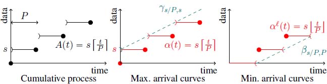
Figure 6.11. A periodic flow and its arrival curves. For a color version of this figure, see www.iste.co.uk/bouillard/calculus.zip
Time-shifted periodic flows. We have just described the idealized shape of a flow. In fact, it is often the case that the flow is not exactly periodic. First, packets might not start to arrive at time 0 exactly, but are time-shifted to ![]() . In that case,
. In that case, ![]() . As
. As ![]() , the maximal arrival curves remain the same as before. Only the minimal arrival curve differs:
, the maximal arrival curves remain the same as before. Only the minimal arrival curve differs: ![]() (the period when no packet in received is at most
(the period when no packet in received is at most ![]() ). These arrival curves are depicted in Figure 6.12.
). These arrival curves are depicted in Figure 6.12.
Periodic flows with jitter. When the behavior of the flow is not ideal, there might also be some jitter in the arrival of packets. This means that the inter-arrival time between packets is not always constant, but lies in some interval (whose length is the jitter). For example, this can be obtained as the departure cumulative process of a periodic flow in a server that has delay guarantees, as in section 6.3.1.2. More formally, there is a period P and a jitter J such that the arrival date of the i-th packet belongs to ![]() . We assume that 0 ≤ J < P. Another definition that can be found in the literature is that the arrival date of the i-th packets belongs to
. We assume that 0 ≤ J < P. Another definition that can be found in the literature is that the arrival date of the i-th packets belongs to ![]() .
.

Figure 6.12. A time-shifted periodic flow and its arrival curves. For a color version of this figure, see www.iste.co.uk/bouillard/calculus.zip
Consider an interval of time d. The number of packets that can arrive during an interval of time d is between ![]() and
and ![]() , and so a maximal arrival curve is
, and so a maximal arrival curve is ![]() and a minimal arrival curve is
and a minimal arrival curve is ![]() . These arrival curves can respectively be approximated by
. These arrival curves can respectively be approximated by ![]() and
and ![]() .
.
Variable packet size. Assume now that each packet can have a different value, in an interval ![]() . Then, such a flow has the same maximal arrival curve
. Then, such a flow has the same maximal arrival curve ![]() and minimal arrival curve
and minimal arrival curve ![]() .
.
These curves can be obtained similarly to the previous section: if at most k packets can arrive during a time interval, then the amount of data that can arrive during that time interval is ksu.
Sporadic flows. Finally, a sporadic flow with pseudo-period P is a flow where there is a minimal inter-arrival time P between any two packets. In that case, only a maximum arrival curve can be computed, which is ![]() .
.
6.3.2.1.2. Propagation and performance bounds
Let us now consider a flow crossing a server offering a min-plus service curve βR,T, which is a λR-shaper. We assume that s/P < R to ensure the stability of the system.
The departure cumulative process D then satisfies ![]() . These bounds are depicted in Figure 6.13.
. These bounds are depicted in Figure 6.13.

Figure 6.13. Periodic flow crossing a rate-latency server
We first apply Theorem 5.2 to the system using the two maximal arrival curves that have been derived: the tighter one (![]() in the most general case) and the linear approximation
in the most general case) and the linear approximation ![]() . We obtain:
. We obtain:
- –
 ;
; - –
 and
and  .
.
Computing the delay upper bound with a staircase arrival curve leads to extensive computations in the general case. In the ideal case (J = 0), the delay obtained is exactly the one obtained in the linear case. This is illustrated in Figure 6.14.

Figure 6.14. Performance bounds for a periodic flow crossing a rate-latency server. For a color version of this figure, see www.iste.co.uk/bouillard/calculus.zip
Let us now consider the arrival curve of the cumulative departure function D. We will only consider the arrival curve α2, since, as stated in section 3.1.1, there is no nice analytic representation when doing the computations with α1. In this latter case, it is still possible to compute an arrival curve using the algorithm procedures described in Chapter 4. Figure 3.2 gives some hints on the shape of the functions.
From Theorem 5.3, the cumulative departure function has arrival curve
6.3.2.2. Shaping and periodic flows
We have just seen that the shape of the arrival curve of the departure process after a server that has a maximum service rate (or a shaper) differs from those of the arrival curves of periodic arrivals. In particular, this is the minimum of a linear function with another arrival curve. Modeling this has a significant impact on performance bounds (approximately 40% in a realistic AFDX configuration [GRI 04]). We call it the shaping effect.
To illustrate this and keep things simple, consider a periodic flow of period P with packet size s that crosses a server with constant rate C. Our aim here is to compute the delay bound of this flow crossing a second server offering a min-plus service curve βR,T, and compare it with the delay that would be obtained without considering the shaping effect. We assume that the system is stable, i.e. s/P < min(C, R).
First, take the token-bucket approximation of the arrival curve ![]() . As stated in the previous section, the arrival curve at the second server is
. As stated in the previous section, the arrival curve at the second server is
This type of arrival curve is used for Traffic Specification (TSpec) [SHE 97], presented in Figure 4.1. In the second server (with min-plus service curve βR,T), the delay bound that can be obtained is therefore

which has to be compared to the delay bound without shaping:
The factor ![]() can be interpreted as a burst reduction factor. Note that when C < R, the delay is T. The comparison is illustrated in Figure 6.15 (left).
can be interpreted as a burst reduction factor. Note that when C < R, the delay is T. The comparison is illustrated in Figure 6.15 (left).
Now consider the tighter arrival curve ![]() . Computations show that
. Computations show that ![]() is an arrival curve for the arrival process in the second server. In fact, a better arrival curve can be computed: from Proposition 5.2 and Proposition 2.6, an arrival curve is
is an arrival curve for the arrival process in the second server. In fact, a better arrival curve can be computed: from Proposition 5.2 and Proposition 2.6, an arrival curve is ![]() . The construction is illustrated in Figure 6.15 (right).
. The construction is illustrated in Figure 6.15 (right).

Figure 6.15. Shaping vs. no shaping of arrival curves. Left: token bucket arrival curve; right: staircase arrival curve. For a color version of this figure, see www.iste.co.uk/bouillard/calculus.zip
6.3.2.3. Arrival curves for pattern-based processes
Until now, we have focused on very simple periodic patterns: one packet arrives every P units of time. Here, we call more general periodic processes pattern-based processes. Such cases occur when a flow is the aggregation of flows with fixed offsets.
Consider a flow with a periodic behavior of period 5 that sends one packet of size 1 at times 1 + 5n and times 4 + 5n, ![]() . Its cumulative arrival process is
. Its cumulative arrival process is ![]() , as depicted on the left-hand side of Figure 6.16. The best arrival curve of this process can be computed as
, as depicted on the left-hand side of Figure 6.16. The best arrival curve of this process can be computed as ![]()
![]() . Intuitively, this is A(t − 4): from time 4, packets arrive the fastest. Note that several linear approximations,
. Intuitively, this is A(t − 4): from time 4, packets arrive the fastest. Note that several linear approximations, ![]() and
and ![]() , can be computed, as illustrated in Figure 6.16. Their minimum is also an arrival curve.
, can be computed, as illustrated in Figure 6.16. Their minimum is also an arrival curve.

Figure 6.16. An example of pattern-based process and its arrival curves. For a color version of this figure, see www.iste.co.uk/bouillard/calculus.zip
This example can be made more complex by considering that odd packets have size 3/2 and even packets size 1/2: the arrival process is ![]() . The arrival curve is not shifted from the process: in an interval of length d ∈ (0, 2], the amount of data arriving is at most 1.5, and during an interval of time d ∈ (2, 5], it is 2. Thus,
. The arrival curve is not shifted from the process: in an interval of length d ∈ (0, 2], the amount of data arriving is at most 1.5, and during an interval of time d ∈ (2, 5], it is 2. Thus, ![]() .
.
6.4. Summary
Server composition: For minimum min-plus or maximum service curves,

Pay burst only once phenomenon: ![]() .
.
Greedy server control: If ![]() , then
, then ![]() .
.
Window flow control: ![]() . If
. If ![]() , then βwfc = β.
, then βwfc = β.
Modeling with service curves:
- – Constant-rate server with rate
 .
. - – Delays:
 .
.
Modeling with arrival curves:
- – Periodic flow with period P, jitter J and packet size in
 :
:
- - max. arrival curves:
 and its linear approximation
  ;
; - - min. arrival curves:
 and its linear approximation
  .
.
- - max. arrival curves:
- – Shaped flow has maximal arrival curve shaped like
 .
.