
|
|


Physical data modeling is the process of capturing the detailed technical solution. This is the first time we are actually concerning ourselves with technology and technology issues such as performance, storage, and security. For example, conceptual data modeling captures the satellite view of the business requirements, revealing that a Customer places many Orders. Logical data modeling captures the detailed business solution, which includes all of the properties of Customer and Order such as the customer’s name, their address, and the order number. After understanding both the high level and detailed business solution, we move on to the technical solution, and physical data modeling may lead to embedding Order within Customer in MongoDB.
In physical data modeling, we aim to build an efficient MongoDB design, addressing questions such as:
- What should the collections look like?
- What is the optimal way to do sharding?
- How can we make this information secure?
- How should we store history?
- How can we answer this business question in less than 300 milliseconds?
Physical Data Modeling Approach
There are five steps to physical data modeling:

Starting with our logical data model, we prepare the initial MongoDB structure by deciding for each relationship whether to embed or reference (Step 1). After making these changes to the model, we can determine where to accommodate history (Step 2). History means keeping track of how things change over time. There most likely will be other structural refinement needed such as adding indexes or sharding; both techniques are used to further improve retrieval performance (Step 3). In Step 4, review the work to get approval. Frequently, action items come out of the review and confirm step where we need go back to Step 1 and refine the structure. Expect iteration through these steps. Once we have received final confirmation from our work, we can move on to implementation. Let’s talk more about each of these five steps.
Step 1: Embed or Reference
MongoDB resolves relationships in one of two ways: embed or reference. Recall from Chapter 3 that embedded documents resolve relationships between data by storing related data in a single document structure, and a reference is a pointer to another document. MongoDB documents make it possible to embed document structures as sub-documents in a field or an array within a document. Embed is equivalent to the concept of denormalization, in which entities are combined into one structure with the goal of creating a more simplistic and performant structure, usually at the cost of extra redundancy and, therefore, storage space. One structure is often easier than five structures from which to retrieve data. Also, the one structure can represent a logical concept such as a survey or invoice or claim.
If I need to retrieve data, it can (most of the time) take more time to get the data out of multiple documents by referencing than by embedding everything into a single document. That is, having everything in one document is often better for retrieval performance than referencing. If I frequently query on both Order and Product, having them in one document would most likely take less time to view than having them in separate documents and having the Order reference the Product.
Notice the language though in the preceding paragraph; “most of the time” and “most likely” imply that embedding is not always faster, nor should retrieval speed be the only factor to consider when deciding whether to embed or reference. The top five reasons for embedding over referencing are:
- Requirements state that data from two or more entities are frequently queried together. If we are often viewing data from multiple entities together, it can make sense to put them into one document. It is important to note that this factor, which is possibly the most important factor in deciding whether to embed or reference, has more to do with usage than technology. No matter how skilled we are with MongoDB, we still need to know the business requirements!
- The child is a dependent entity. In the following model, Customer and Account in Example 1, and Customer in the Example 2 are independent entities (shown as rectangles), and Account in Example 2 is a dependent entity (shown as a rectangle with rounded corners).

An independent entity is an entity where each occurrence (instance) can be found using only its own attributes such as a Customer ID for Customer. A dependent entity, such as Account in the second example, contains instances that can only be found by using at least one attribute from a different entity such as Customer ID from Customer.
To make the explanation of independent and dependent clearer, here are our two data models with example values for two attributes within Account, Account Number and the foreign key back to Customer, Customer ID.

On the model in Example 1, we see that Account Number is unique, and therefore to retrieve a specific Account requires only knowing the Account Number and not anything from Customer, making Account an independent entity because Account Number belongs to Account. However, in Example 2, Account Number 34 appears three times, so the only way to find a specific account is to know who the customer is. So the combination of Customer ID and Account Number is required to distinguish a particular account, making Account in Example 2 a dependent entity because Customer ID, which is needed to help identify accounts, does not belong to Account.
Notice also that the relationship line looks different when connecting to an independent verses dependent entity. The dotted line means non-identifying and the solid line means identifying. Identifying relationships mean that the entity on the many side (the child) is always going to be a dependent entity (like Account in Example 2) to the entity on the one side (the parent).
If we are designing a MongoDB database and trying to decide whether we should embed documents or reference other documents, a major factor would be whether the relationship is identifying or non-identifying. An identifying relationship is a much stronger relationship than non-identifying, giving us more weight towards embedding the weak entity within the strong entity so that we have just one document.
- There is a one-to-one relationship between two entities. A one-to-one relationship means that for a given entity instance, there can be at most one entity instance relating to it, meaning if we decide to embed, there will be no redundancies, thus creating a simple easy-to-query structure. In this model, we would embed Address into Customer:

- Similar volatility. If the entity you are considering embedding within another entity experiences updates, inserts, and deletes at a similar rate to the entity it will be embedded into, there is a stronger reason to combine them. The opposite is the argument for referencing. That is, if you are considering embedding Customer Contact into Customer and Customer Contact information experiences almost hourly changes while Customer is relatively stable, there is a greater tendency towards referencing Customer from Customer Contact instead of embedding. This volatility factor also includes considering chronology requirements. That is, if there is a requirement to store all history (e.g. auditing) on one entity but a current view only on the other entity, you may lean towards referencing over embedding.
- If the entity you are considering embedding is not a key entity. If Claim and Member have a relationship but Claim has many other relationships, it may be prudent to reference Member from Claim instead of embedding the key entity Claim into Member. It is more efficient and less error prone to reference the entity that is needed by many other entities. Another example are many-to-many relationships where the associative entity (the entity that resolves the many-to-many), is referenced by at least two other entities. In these situations it may be better to reference rather than embed. For example, I would not consider embedding entity B into any of the other entities on this model (I might consider embedding one or a few of the surrounding entities into B, however):

Two more points on embedding versus referencing:
- If some of these five factors apply but others don’t, the best option is to test both ways (embed and reference) and go with the one that gives the best results, where results include retrieval performance, ease of data updates, and storage efficiencies. Because we are working without predefined schemas, it is a lot easier to test in MongoDB than in a relational database environment.
- MongoDB imposes a size limit on a single document of 16 MB. It is very unlikely the size factor will influence your decision as to whether to embed or reference, as this is a huge amount of space (e.g. 120 million tweets), and therefore this factor rarely becomes a decision point. In addition, MongoDB arrays that grow very large tend to perform poorly even when indexed. If a set of values or sub-documents will grow significantly over time, consider referencing over embedding to avoid this performance penalty.5
EXERCISE 7: Embed or Reference
Below are two scenarios with accompanying data models. Based on the scenario and the sample MongoDB document, decide whether you would embed or reference. Please see Appendix A for my responses.
|
Scenario |
Sample Embedded Document |
Sample Referenced Document |
|
We are building an application that allows easy querying of customers and their accounts. Customer has lots of other relationships, and in this scenario Account has no other relationships.
|
Customer : { _id : "bob", customerName : "Bob Jones", customerDateOfBirth : ISODate("1973-10-07"), accounts : [ { accountCode : "3281", accountOpenDate : ISODate("2014-02-05") }, { accountCode : "12341", accountOpenDate : ISODate("2014-03-21") } ] } |
Customer : { _id : "bob", customerName : "Bob Jones", customerDateOfBirth : ISODate("1973-10-07") } Account : { customerId : "bob", accountCode : "3281", accountOpenDate : ISODate("2014-02-05") } Account : { customerId : "bob", accountCode : "12341", accountOpenDate : ISODate("2014-03-21") } |
|
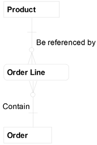
We are building an application to allow efficient data entry of product order information. Order contains over 100 fields, Order Line contains over 50 fields, and Product contains over 150 fields. An Order, on average, contains 20 Order Lines. Would you embed Order Line into Order?
|
Order : { _id : "1234", orderNumber : "AB-3429-01", orderDate : ISODate("2013-11-08") }, orderLines : [ { orderLineSequenceNumber : "1", productId : "2837", orderLineQuantity : 15 }, { orderLineSequenceNumber : "2", productId : "2842", orderLineQuantity : 25 } ] } |
Order : { _id : "1234", orderNumber : "AB-3429-01", ISODate("2013-11-08") } OrderLine : { orderId : "1234", orderLineSequenceNumber : "1", productId : "2837", orderLineQuantity : 15 } OrderLine : { orderId : "1234", orderLineSequenceNumber : "2", productId : "2842", orderLineQuantity : 25 } |

Recall from this section’s introduction that relational data modeling is the process of capturing how the business works by precisely representing business rules, while dimensional data modeling is the process of capturing how the business is monitored by precisely representing business questions. The thought process for this step is the same for both relational and dimensional physical data modeling, so let’s look at an example of each.
For Relational
On the facing page is our relational logical data model from Chapter 6. I would take a pencil and start grouping the logical entities together that I think would make efficient collections.

Here are my thoughts during this grouping process:
- The subtypes are dependent entities to their supertype, and therefore frequently we roll subtypes up to supertypes and add type codes to the supertype such as customerTypeCode and accountTypeCode.
- We have a one-to-one relationship between Check and CheckDebit, which is a great candidate, therefore, for embedding Check into CheckDebit.
- The documents, such as WithdrawalSlip, and their corresponding transactions, such as WithdrawalDebit, have similar volatility and therefore are good candidates for embedding. I would not initially embed these transactions and documents into Account because of the high difference in volatility with Account. We might have millions of transactions, yet only 1,000 accounts that change on a regular basis, for example.
- Assuming stable branch data, we can embed Branch in Account.
- For now, Customer and Account remain separate collections. Often many-to-many relationships become references instead of embedded collections because of the complexities of storing a complex relationship in one structure.
Here is the completed relational PDM after making these changes:

For Dimensional
A star schema is the most common physical dimensional data model structure. The term meter from the dimensional logical data model, is replaced with the term fact table on the dimensional physical data model. A star schema results when each set of tables that make up a dimension is flattened into a single table. The fact table is in the center of the model, and each of the dimensions relate to the fact table at the lowest level of detail.
Recall the dimensional logical data model example from the last chapter:

Let’s convert this to a star schema:

Notice I used a physical dimensional modeling technique called a degenerate dimension in this example. A degenerate dimension is when you remove the dimensional structure and just store the dimensional attribute directly in the fact table. Most of the time, the degenerate dimension contains just a single field—in this case, an indicator. So we removed those dimensions such as University that contained only a single field.
Step 2: Accommodate History
There are four options in addressing how field values change over time. Each option for handling these changes is given a different number (either zero, one, two, or three) and is often called a Slowly Changing Dimension (SCD for short). An SCD of Type 0 means we are only storing the original state and not storing changes. That is, a collection of Type 0 means that if the data changes, we just store the way the data was originally and do not apply any changes to it. A Type 1 means the most current view. With a Type 1 we are just storing the most current state of the collection by applying the latest changes. A Type 2 means we are storing all changes to the data in a collection—a complete history whenever anything changes. Type 2 is also known as “auditing” because we are storing all changes and therefore have the ability to analyze the way the world existed at any point in time. Type 2 is like having a time machine. Type 3 means we have a requirement for some history—for example, the most current view and the previous view or the most current view and the original view.
We need to determine the type of history needed for each collection by completing the Collection History Template:
Collection History Template
|
Store only the original state (Type 0) |
Store only the most current state (Type 1) |
Store full history (Type 2) |
Store some history (Type 3) |
|
|
Collection A |
||||
|
Collection B |
||||
|
Collection C |
Note that it is not uncommon for a collection to have more than type of history requirement such as Customer requiring a Type 1 for customerLastName and a Type 2 for emailAddress. Also, the thought process for this step is the same for both relational and dimensional physical data modeling, so let’s look at an example of each.
For Relational
Here is the completed Collection History Template for our Account example:
Account Project Collection History
|
Store only the original state (Type 0) |
Store only the most current state (Type 1) |
Store full history (Type 2) |
Store some history (Type 3) |
|
|
Customer |
✓ |
|||
|
AccountOwnership |
✓ |
|||
|
Account |
✓ |
|||
|
WithdrawalDebit |
✓ |
|||
|
DepositCredit |
✓ |
|||
|
InterestCredit |
✓ |
|||
|
CheckDebit |
✓ |
|||
|
BankAccountStatement |
✓ |
Note that transactions and documents are often created but rarely change, which is why a Type 1 is chosen. Note also that it is common to have a Type 2 on Customer and Account. There are a number of ways to model a Type 2, the most common being to put an effective date in the entity’s primary key:

There are other ways of modeling a Type 2, some of which are more efficient for child entities, such as WithdrawalDebit, which now has a larger and more complex primary key.
For Dimensional
Here is the completed Collection History Template for our University example:
Student Attrition Collection History
|
Store only the original state (Type 0) |
Store only the most current state (Type 1) |
Store full history (Type 2) |
Store some history (Type 3) |
|
|
Department |
✓ |
|||
|
Calendar |
✓ |
Note that because Type 1 is requested for both Department and Calendar, our data model does not need to change and remains with the same structure as our prior step:

Step 3: Index and Shard
The primary and alternate keys from our logical data model are converted into unique indexes on the physical. We can also add additional indexes for performance, called secondary or non-unique indexes. For example, if there is a continuous need to see customerLastName and customerFirstName, we can add indexes to these fields to reduce the amount of time it takes to retrieve.
Partitioning (called “sharding” in MongoDB) is when a document is split up into two or more parts. Vertical partitioning is when fields are split up and horizontal is when documents are split up. Frequently, both horizontal and vertical are used together. That is, when splitting documents apart, in many cases we learn that certain fields only belong with certain documents.
Both vertical and horizontal partitioning are common techniques when building analytics systems. A collection might contain a large number of fields and perhaps only a subset are volatile and change often, so this subset can be vertically partitioned into a separate collection. Or we might have ten years of orders in a table, so to improve query performance we horizontally partition by year so that when queries are run within a given year, the performance will be much faster.
For Relational
For our relational physical data model, these attributes are queried frequently and therefore need non-unique indexes: customerFirstName and customerLastName (we added a composite index6 on both of these attributes), customerTypeCode, accountTypeCode, branchCode, and accountName:

For Dimensional
For our dimensional physical data model, these attributes are queried frequently and therefore need non-unique indexes: departmentName, yearCode, and semesterCode:

Step 4: Review and Confirm
Previously, we identified the person or group responsible for validating the model. Now we need to show them the model and make sure it is correct. Often at this stage after reviewing the model, we go back to Step 1 and make some changes and then show the model again. This iterative cycle continues until the model is agreed upon by the validator and deemed correct so that we can move on to MongoDB implementation.
Step 5: Implement
We’re done with our modeling, and now we can start creating documents within each of these collections!
|
Key Points
|