Appendix 2
Matrix Representation of a Dioptric System
The objective of this time-harmonic representation is to express the amplitudes of bulk waves that propagate in a solid occupying the half-space x2 > 0. These amplitudes are expressed as a function of the mechanical quantities that are conserved at an interface, that is, the three components of mechanical displacement u and those of mechanical traction: ![]() for a surface of normal l parallel to the x2 axis. The phenomena associated with the emission, detection and diffraction of elastic waves can be formulated using a mixed matrix M, whereby the vector b for the amplitudes of the reflected (emitted) bulk waves and the mechanical amplitude u on the surface is related to the vector a for the amplitudes of the incident bulk waves and to the mechanical traction T. This matrix M consists of four sub-matrices D, E, R and Y :
for a surface of normal l parallel to the x2 axis. The phenomena associated with the emission, detection and diffraction of elastic waves can be formulated using a mixed matrix M, whereby the vector b for the amplitudes of the reflected (emitted) bulk waves and the mechanical amplitude u on the surface is related to the vector a for the amplitudes of the incident bulk waves and to the mechanical traction T. This matrix M consists of four sub-matrices D, E, R and Y :

Generally, the vectors a and b have three components (one for each bulk wave), and the vectors u and T also have three components:

The sub-matrices are thus square (3 × 3) matrices:
- – the diffraction matrix D provides the amplitudes of reflected waves as functions of the amplitudes of the incident waves when the surface is free (T= 0 );
- – the emission matrix E gives, in the absence of incident waves (a= 0 ), the amplitudes b of bulk waves created by a uniform distribution of forces T on the surface;
- – the reception matrix R is useful for calculating the mechanical displacement u induced, on the free surface (T= 0 ), by bulk waves of amplitude a;
- – the admittance matrix Y gives, in the harmonic case, the mechanical displacement created by a uniform distribution of forces exerted on the surface. The components of its Fourier transform are the Green’s functions of the half-space for mechanical surface phenomena.
A2.1. Diffraction matrix
Consider an incident, homogeneous plane wave of amplitude a, whose polarization is defined by the unit vector p. For transversely independent problems, the wave vector k is contained in the x1x2 plane:
Upon omitting the propagation factor, the stresses σi2 are in the form:

By introducing the dimensionless parameters m = k2/k1, which defines the propagation direction in the x1x2 plane, the mechanical traction involved in the boundary conditions on the surface x2 = 0 is given by:
The mechanical traction on the surface is the sum of those created by each incident wave (denoted by the index I = 1, 2, 3); by writing ti = Ti/ik1 :

where A = [AiI] is the (3 × 3) matrix obtained by juxtaposing the column vectors AI of each incident bulk wave. Identical considerations for the reflected waves (denoted by the index J = 1, 2, 3), of amplitude b and unit polarization q, lead to the definition of the matrix B such that:
The total mechanical traction is given by the sum:
Since t = 0 on the free surface x2 = 0, the amplitudes of the reflected bulk waves are expressed as functions of the amplitudes of the incident waves by:
The nine components of the diffraction matrix D are the reflection coefficients. For example, by attributing the index 1 to the quasi-longitudinal (QL) wave and the indices 2 and 3 to the quasi-transverse (QT) waves, the vector a= (a1, 0, 0)t represents an incident QL wave of amplitude a1. The components of the first row in the matrix D are the reflection coefficients into the QL wave (r11 = b1/a1) and the conversion coefficient into the QT wave (r12 = b2/a1, r13 = b3/a1). According to the matrix inversion rule:

the denominator for all the reflection coefficients is the determinant of the matrix B.
In the absence of any incident wave (a= 0 ), the homogeneous system Bb = 0 has a non-trivial solution if:
An elastic wave with non-zero displacement b can propagate on the free surface of a solid. This wave was discovered in the case of an isotropic solid by Lord Rayleigh in 1885. The characteristic equation of a Rayleigh wave is therefore obtained by canceling the denominator of the reflection coefficients on the free surface of an isotropic solid. This observation can also be applied to waves that propagate along the interface between a fluid and a solid, or between two solids, whether isotropic or anisotropic.
A2.2. Emission, admittance and reception matrices
In the absence of any incident wave (a= 0 ) and according to relation [A2.8]: b = B−1t, the amplitudes b of the emitted bulk waves are expressed as functions of the stress vector T on the surface, using the emission matrix E:
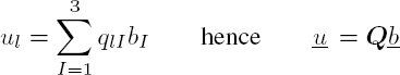
With Q = [qlJ] denoting the polarization matrix of the emitted (reflected) waves, the mechanical displacement on the surface:
can be expressed as a function of the stress vector T using the admittance matrix Y :
By using P = [plI] to denote the polarization matrix of incident waves, the total mechanical displacement on the surface created by the incident waves of amplitude a, and reflected waves of amplitude b= B−1Aa, is expressed using the reception matrix R:
A2.3. Isotropic solid
Given that only two bulk waves can propagate in an isotropic solid and for the displacements u and mechanical tractions T contained in the (x1, x2) plane, the sub-matrices of the mixed matrix are (2 × 2) matrices. According to the Snell–Descartes law, the component s1 of the slowness vector is identical for all waves and s3 = 0. The normal components s2L and s2T are given by the dispersion relations:
where sL = 1/VL and sT = 1/VT are the slownesses of longitudinal and transverse waves. The development of relation [A2.4] for the emitted waves, of amplitude b and of polarization vector q:
with C22 = C11 and C21 = C11 − 2C66, leads to:
For the longitudinal wave, the normalized components ![]() of the polarization vector are:
of the polarization vector are:
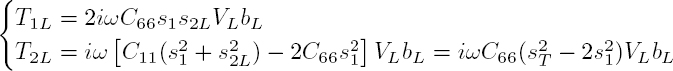
Using the relation ![]() the components of mechanical traction TL are given by:
the components of mechanical traction TL are given by:
Similarly, for the transverse wave:
the components of the mechanical traction TT are written as:

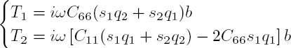
By introducing the Lamé constant μ = C66, the stress vector T = TL + TT is written in matrix form as:

The inversion leads to the emission matrix:

where Δ is the Rayleigh determinant:
Considering relations [A2.19] and [A2.21], the polarization matrix of the reflected or emitted waves is:

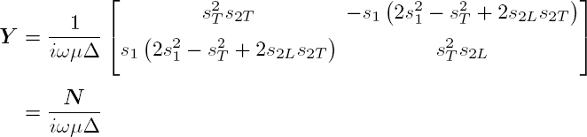
and the admittance matrix Y can be deduced from relation [A2.14] Y = QE, with: