
1
Radiation of Elastic Waves
Acoustic waves emitted by sources of finite dimensions diverge, so that acoustic pressure and power density decrease with the distance from the transmitter. Understanding the radiation of sources is therefore essential to predict the acoustic field emitted by transducers used for medical diagnosis or in sonar systems, as well as in defect detectors in metallurgy or in other instruments and sensors.
The chapter is divided into three sections. In the first section, we study the acoustic radiation in a perfect fluid by a vibrating plane surface, then by a focused transducer. In the harmonic case and in a medium where the acoustic wave is defined by a scalar quantity such as the velocity potential or the acoustic pressure, the results are similar to those of the scalar theory of diffraction in optics. One specificity of acoustics is the use of short impulse waves or wave trains of varying durations. By drastically reducing the interferences between the waves emitted by the different points of the source, the conditions of the impulse diffraction, presented at the end of this section, are very different from those observed for time-harmonic waves. In the second section, we analyze the radiation of bulk elastic waves and Rayleigh waves in isotropic or anisotropic solids. With the exception of the explosive sources used in the field of oil exploration, these sources are most often located on the solid surface. The modeling of a seismic or a thermoelastic source is examined in the case of a linear distribution of impulsive forces. The last section is devoted to the radiation from an elementary spherical source embedded in an isotropic solid.
1.1. Acoustic radiation in a fluid
In a perfect fluid and assuming that the wave is a small perturbation of the reference state (pressure p0, mass density ρ0), the acoustic pressure pa = p − p0 and the particle velocity v are solutions to the local equation of dynamics, also called the linearized Euler equation:
and to equation [1.322] from Volume 1:
resulting from the linearization of the continuity equation and the pressure–density relation of the fluid. F (x, t) is the force density per unit mass and c is the sound speed. In order to solve this system of first-order partial differential equations, it is convenient to express the acoustic pressure and particle velocity in terms of a single scalar function, the velocity potential φ(x, t), defined by:
In the absence of sources in the volume (F = 0), the acoustic pressure can be deduced from equation [1.1]:
The time-derivation of equation [1.1] shows that the potential φ satisfies the equation:
By introducing the potential s(x, t) of the volume sources, defined by:
equation [1.5] takes the form:
In the harmonic case, the velocity potential and volume source potential vary as e−iωt:
The spectral components Φ(x, ω) and S(x, ω), at angular frequency ω, satisfy the Helmholtz equation:
where k = ω/c is the wave number.
1.1.1. Integral formulation of the Helmholtz equation
The determination of the velocity potential1 Φ(x ) in a closed domain is not always easy. One way to do this is based on the integral formulation of the Helmholtz equation, also called Kirchhoff–Helmholtz equation.
Let us consider a volume V delimited by a surface S of unit normal n, oriented toward outside. The potential Φ(x), which is the solution to the Helmholtz equation [1.9], satisfies known boundary conditions on the surface S (Figure 1.1).
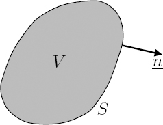
Figure 1.1. Volume V delimited by the boundary S of outer unit normal n
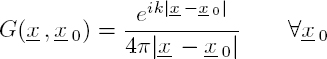
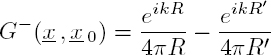
Let G(x, x0) be the Green’s function, solution to the Helmholtz equation in the domain V , whose source term is a Dirac delta function at x0:
The Green’s function verifies the reciprocity principle, which is expressed by the relation:
Multiplying equation [1.9] by G(x, x0), and equation [1.10] by Φ(x) and subtracting both results, we obtain:
The integration of this equation over the volume V leads to the expression:
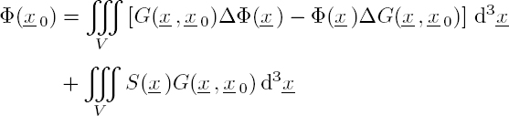
or again, after using the second Green’s identity:
where ∂Φ(x)/∂n is the derivative of the function Φ(x) in the direction of the outgoing normal. By switching the variables x and x0 and considering the reciprocity principle [1.11]:
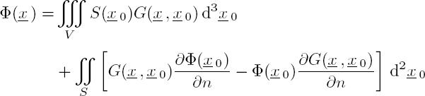
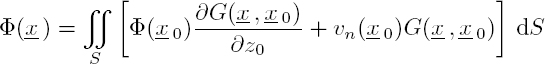
the scalar potential Φ(x) is the sum of two integrals with different properties. The volume integral expresses the acoustic field generated by “primary” sources located inside the volume V . This integral is the convolution product of the Green’s function G(x, x0) with the source function S(x0). The surface integral expresses the effect of the boundary S of the domain on the acoustic field. This allows us to directly integrate the boundary conditions into the propagation equation, which can be useful in the case of complex surfaces, such as non-planar, irregular or vibrating surfaces. However, the analytical calculation of this integral can be difficult. Consequently, it is often carried out numerically.
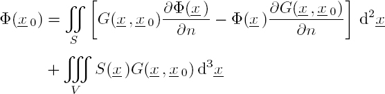
1.1.2. Rayleigh integral
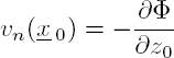
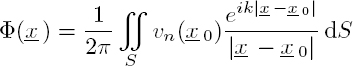
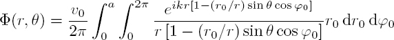
The objective of this section is to determine the field radiated by a plane surface S0, whose points vibrate with the normal velocity vn(x0)e−iωt. The semi-infinite space z > 0, filled with a fluid, is bounded by the infinite plane S located at z = 0. This perfectly rigid plane S contains the emitting surface S0. By hypothesis, the half-space z > 0 is free from volume source, so that the volume integral in equation [1.15] is zero. The velocity potential radiated by the surface S0 of inner normal ez is given by the surface integral2:
which expresses the Kirchhoff–Helmholtz theorem.
Given the relation [1.3] between the particle velocity and the potential Φ, the continuity of the normal velocity imposes:
The velocity potential at point x takes the form:
In the absence of any information on the value of the velocity potential on the surface S and in order to remove the term Φ(x0) in the integral equation, we must find a Green’s function satisfying a Neumann condition (∂G/∂z0 = 0) on this surface. The appropriate Green’s function is obtained using the image-source method, by the summation of the free field Green’s functions (Bruneau 2006):
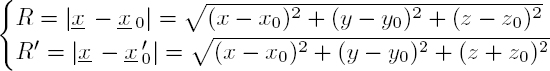
corresponding to a source located at point x0 and to the source image, with respect to the plane z = 0, located at x′0 (Figure 1.2):
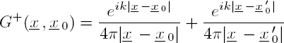
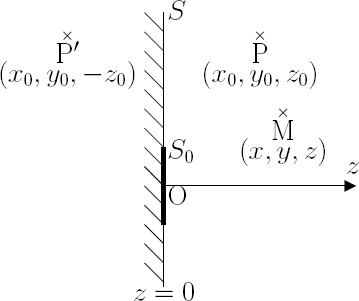
Figure 1.2. Representation of the observation point M, the source P and the image source P′
By writing:
the derivative of the Green’s function with respect to the normal to the surface z = 0 is given by:

or again, considering expressions [1.21] for R and R′:

At z0 = 0, the distances R and R′ are equal and therefore the normal derivative of the Green’s function is zero on the surface z0 = 0. The Green’s function G+ satisfies a Neumann condition on the surface S. Taking into account this condition and the expression [1.20] for a source point located at z0 = 0:

relation [1.18] can be written in the form of the Rayleigh integral:
The Rayleigh integral was established in the harmonic case under the hypothesis that all points on the emitting surface S0 vibrate in phase with a normal velocity vn(x0)e−iωt, a priori non-uniform. In the piston mode, the amplitude distribution can be weighted by a function Pn(x0), which is smooth enough to reduce the edge effects and thus the level of the side lobes. In the uniform piston mode, all the points on the source have the same velocity v0(t); the function Pn(x0) is constant and chosen to be equal to unity on the surface S0, and it is zero outside.
This distinction is independent of the type of excitation, that is, of the operating regime (harmonic, impulse, transient, etc.), as shown in Table 1.1.
Table 1.1. Piston mode: main operating regimes
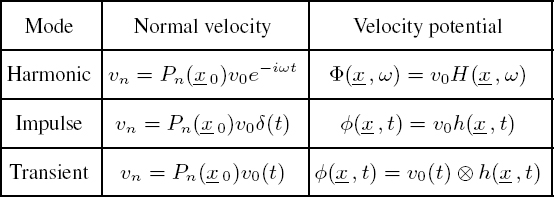
REMARK.– The velocity potential Φ(x, ω) is naturally the Fourier transform of φ(x, t). It is the same for the frequency response H(x, ω) and the impulse response h(x, t).
There exists another operating mode specific to multi-element antennas (or arrays) used in sonars or ultrasound scanners. The source consists of a large number of piezoelectric components, usually rectangular, whose width is small compared to the wavelength. The electric voltage applied to each element is either delayed (in the impulse regime) or phase-shifted (in the harmonic case) according to a linear law, depending on the position of the elements (section 1.1.4.4). The electronic control of the delay or of the phase-shift law ensures the dynamic scanning of these ultrasound imaging devices.
1.1.3. Rayleigh–Sommerfeld integral
If we choose the difference of the free field Green’s functions, the Green’s function obtained:
is zero at any point on the plane surface S, because R = R′ when z0 = 0. By changing the + sign to the – sign in the right-hand side of equation [1.23], the normal derivative to the surface S is expressed as:

Let us carry out two approximations, justified in optics, to calculate the field diffracted by an aperture:
- – the incident wave is little modified on the surface of the aperture, whose dimensions are large with respect to the wavelength λ;
- – the observation point M is located at a large distance, that is, kR >> 1.
Under these conditions, equation [1.18] takes the form:
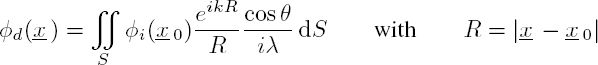
where θ is the angle between the vector x − x0 and the z axis (cos θ = z/R). This Rayleigh–Sommerfeld formula provides the field φd(x) diffracted by a plane aperture over which the incident field φi(x0) is known. This mathematically expresses the Huygens–Fresnel principle, by giving a value cos θ/iλ to the complex amplitude of the hemispherical wavelets emitted, in the propagation direction of the incident wave, at each point on the diffracting surface. The comparison between the Rayleigh integral and the Rayleigh–Sommerfeld integral explains the similarity between the acoustic radiation of a uniform piston [vn(x0) = Const.] at a large distance (R >> λ) and the diffraction of a plane light wave [φi(x0) = Const.] through an aperture whose shape is identical to that of the piston.
1.1.4. Harmonic case
We start by analyzing the radiation of time-harmonic acoustic waves by planar sources such as a circular disk, a rectangular element, or a multi-element linear antenna. These reference sources serve as a model for piezoelectric transducers used in various fields, such as non-destructive evaluation of materials, medical echography and underwater exploration by ultrasound.
1.1.4.1. Plane circular piston
The case of a plane baffled piston is a major problem in acoustics, as it allows us to model many acoustic sources, such as loudspeakers or piezoelectric transducers. The circular source of radius a, vibrating uniformly, is included in an infinite rigid screen (Figure 1.3). The calculation of the Rayleigh integral requires the use of polar and spherical coordinates. The position of a source point P on the surface of the disk is defined by the vector x0 = (r0 cos ϕ0, r0 sin ϕ0, 0) and the observation point M in the domain V is marked by the vector x= (r cos ϕ sin θ, r sin ϕ sin θ, r cos θ).
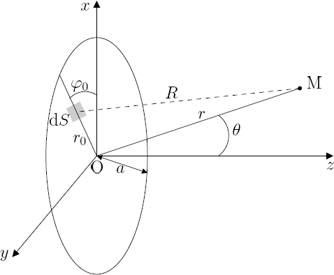
Figure 1.3. The particle velocity on the disk is uniform (constant amplitude v0). The observation point M is assumed to be in the xz plane
The particle velocity, normal to the plane surface, is assumed to be uniform:
Since the problem is axisymmetric, calculations can be performed by taking ϕ = 0, without any loss of generality. The distance R = |x – x0| between the source point and the observation point is equal to:

and the potential at the observation point M is given by:

This integral cannot be expressed analytically in the general case, but it is possible to evaluate it exactly along the piston axis and approximately in the far field.
1.1.4.2. Radiated field on the piston axis
In the harmonic case, the acoustic pressure Pa(x, ω) is related to the velocity potential through relation [1.4]:
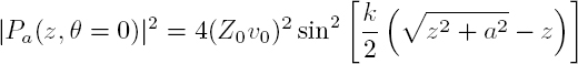
where Z0 = ρ0c is the acoustic impedance of the fluid. On the piston axis (θ = 0), this pressure can be expressed as:

By performing the change of variable ![]() , the acoustic pressure takes the form:
, the acoustic pressure takes the form:

Thus, the pressure field results from the interference of a traveling plane wave emitted by the whole piston, and a wave generated by diffraction on the edge of the piston.
The amplitude of the pressure field normalized by Z0v0 is plotted in Figure 1.4, as a function of the ratio z/a for four different values of the product ka: (a) ka = 1, (b) ka = 10, (c) ka = 50 and (d) ka = 100. For ka = 1, that is, when the wavelength λ = 2πa is larger than the piston radius, the acoustic pressure on the piston axis decreases rapidly. If the wavelength is comparable to the radius (ka = 10), this pressure passes through a single maximum and then decreases as z increases. In situations where the radius a is greater than the wavelength λ, the amplitude of the normalized pressure oscillates between 0 and 2 and then subsequently decreases. The larger the product ka is, the greater the number of oscillations in the near field. The position of the last maximum marks the limit between the Fresnel zone, representing the near field, and the Fraunhofer zone, representing the far field.

Figure 1.4. Amplitude of the normalized pressure field radiated by a uniform piston of radius a along its axis for four values of the product ka
1.1.4.2.1. Near field: Fresnel zone
The positions of the pressure maxima and zeros are easily deduced from its modulus. According to relation [1.34]:
the expression for the modulus of the pressure normalized by Z0v0 is:

The pressure maxima result from constructive interference. They correspond to the extreme values of the sine function:
therefore, for the values of z that satisfy relation:
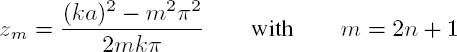
The maximum that is farthest from the source is located at the distance z1 (m = 1):
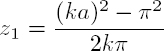
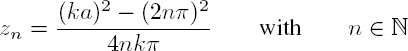
The pressure cancellations result from destructive interference, which takes place when the argument of the sine is equal to nπ, that is, for values of zn that satisfy relation:
1.1.4.2.2. Far field: Fraunhofer zone
The position of the last pressure maximum is often used as the lower limit of the far field. If the piston radiates at high frequency, the product ka is large and the position of the last pressure maximum is:

This expression remains valid as long as the distance z between the far field input and the source is large compared to the source diameter and to the wavelength.
ORDER OF MAGNITUDE.– In immersion experiments, it may be important to place the sample to be probed in the far field of the emitter. For a transducer of diameter 2a = 13 mm, which generates longitudinal waves in water at a frequency f = 10 MHz, the far field corresponds to z > a2/λ ≈ 28 cm.
In the far field, the distance z is large in front of the radius a. A limited development over the quantity ![]() shows that the pressure decreases as 1/z:
shows that the pressure decreases as 1/z:

1.1.4.3. Directivity in the far field
As previously mentioned, the Fraunhofer zone corresponds to the far field, that is, to distances r larger than the radius a of the piston. In this case, the distance |x – x0| appearing in the expression [1.31] of the velocity potential can be approximated by:

so that:
or again:
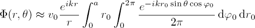
Knowing that the zero-order and first-order cylindrical Bessel functions satisfy the relations:

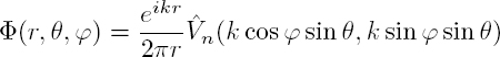
with x = kr0 sin θ, the velocity potential takes the form:
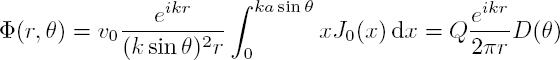
Q = πa2v0 is the piston flow and D(θ) is the directivity factor, given by:
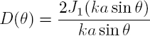
Since J1(x) = x/2 for small values of x = ka sin θ, the function D(θ) is maximal and equal to unity for θ = 0.
In Figure 1.5, the directivity factor is plotted for two values of the product ka. If ka is small compared to unity, that is, at low frequency, the directivity factor is close to unity and depends little on θ. The radiation is omnidirectional and the source behaves like a point source (which is in agreement with the fact that its dimensions are small compared to the wavelength). When the product ka increases, the number of side lobes increases and the width of the main lobe shrinks: the piston is more directional at high frequency.
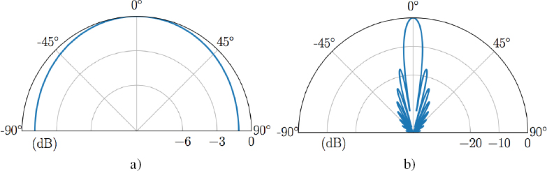
Figure 1.5. Directivity patterns of a circular piston of radius a for a) ka = 1 and b) ka = 25. The level of the first side lobe is 17.5 dB below that of the main lobe
Two parameters are used to characterize the directivity of the emitted acoustic beam:
- – The divergence angle defined by the angular difference 2θ0 between the zeros on either side of the main lobe. Knowing that the first zero of the Bessel function J1(x) corresponds to the argument x = 3.83, the divergence angle of the beam is given by:
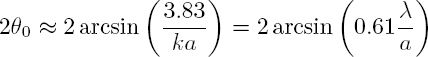
Since the maximum of the first side lobe is equal to only 0.133, that is –17 dB relative to that of the central lobe, the energy emitted by the disk is contained, for the most part, in the cone of apex angle 2θ0 ≈ 1.22λ/a, if λ << a.
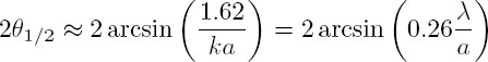
- – The –3 dB angular aperture is defined by the angular difference 2θ1/2 between the two directions (in a meridian plane) for which the acoustic power is divided by two. It is twice the angle θ1/2 for which the directivity factor is divided by
 that is,
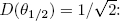
The emission by the piston disk is more directional when its diameter 2a is large with respect to the wavelength λ.
1.1.4.4. Linear array
The antennas (transmitters and receivers) of underwater exploration and localization systems (sonar) or the arrays of medical ultrasound equipment are made up of a large number of rectangular piezeoelectric elements. The direction of the emitted acoustic beam is controlled by applying a delay law or a phase law to the different elements. The angular width of the swept sector is limited by the aperture of the beam emitted by an isolated element, whose width must be smaller than the wavelength λ. The angular resolution is all the better as the length L of the antenna is large compared to λ. Therefore, the number 2N of elements of the antenna must be large, typically 32 ≤ 2N ≤ 256.
1.1.4.4.1. Rectangular element
Let us first examine the acoustic radiation in the far field of a rectangular element of width 2d (along x) and height 2h (along y), located at z = 0 and included in the surface S (Figure 1.6). A point on its surface S0 is defined by the vector x0 = (x0, y0, 0), where x0 ∈ [–d, d] and y0 ∈ [–h, h]. An observation point M is marked in the domain V by the vector x= (r cos ϕ sin θ, r sin ϕ sin θ, r cos θ).

Figure 1.6. Uniform rectangular element of width 2d, height 2h and area S0 = 4dh. The field is calculated at the position x = OM
Assuming that x0 and y0 are small compared to r, the norm of vector |x – x0| is expressed by:
In the harmonic case, the velocity potential results from the Rayleigh integral [1.25]; in the far field, its approximate expression becomes:

Since the vibratory velocity vn is zero in the plane S, removed from S0, the bounds of the two integrals can be extended to infinity. The velocity potential is then given by
where ![]() is the double spatial Fourier transform, defined by the relation:
is the double spatial Fourier transform, defined by the relation:

This formulation is general: in the far field, the velocity potential emitted by a plane surface S vibrating in the piston mode (vn = v0Pn(x0)) is proportional to the spatial Fourier transform of the amplitude distribution Pn(x0) of the normal velocity:

Thus, the expression [1.45] for the acoustic field radiated by the uniform circular piston in Figure 1.3 can be found directly. In the xz plane (ϕ = 0), equivalent to any plane due to the symmetry of revolution: kx = k sin θ, ky = 0, we obtain with x0 = r0 cos ϕ0:

where D(θ) is the directivity factor [1.48].
If the rectangular element vibrates in a uniform piston mode, the normal velocity is independent of the point:

The expression for the velocity potential is:
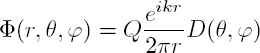
where Q = 4dhv0 is the piston flow and the directivity factor D(θ, ϕ) is a double cardinal sine function:
The radiation in the far field of a rectangular element of width 2d = 1 mm and height 2h = 3 mm vibrating at 10 MHz is represented in Figure 1.7. The field is calculated at a distance r = 50 mm. The color scale is saturated in order to visualize the side lobes.

Figure 1.7. Radiation in the far field (r = 50 mm) of a plane rectangular piston, of dimensions 2d = 1 mm and 2h = 3 mm, at a frequency f = 10 MHz. For a color version of this figure, see www.iste.co.uk/royer/waves2.zip
1.1.4.4.2. Linear antenna
Let us now consider the case of a distribution of 2N linear rectangular elements of width 2d and height 2h (Figure 1.8). The velocity potential is given by the relation:

with, in the far field:
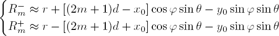

Figure 1.8. Linear antenna composed of 2Nsources aligned along the x axis
In order for the plane P, inclined at an angle β with respect to the normal, to be equiphase, it is necessary to compensate the phase difference Δψ = 2kd sin β between waves emitted by two adjacent elements, 2d apart, by applying to the emission a phase law ψm = ψ0 – kxm sin β, linear versus the abscissa xm = ±(2m + 1)d. Assuming that each element radiates with the same flow Q and with a uniform velocity equal to:
the velocity potential in the xz plane (ϕ = 0) takes the form:
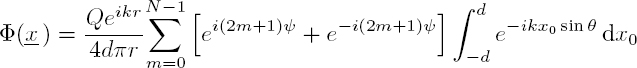
with ψ = kd(sin θ sinβ). Given expression [1.59] for the directivity factor of a rectangular element:
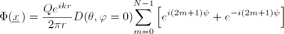
and by recognizing the geometric series Σm qm, we obtain:

In Figure 1.9, the radiation pattern for a linear antenna composed of 2N = 64 rectangular elements, of width 2d = 4 mm and height 2h = 4 cm, is plotted in the xz plane (ϕ = 0) as a function of angle θ for three phase-shift angles: β = 0◦, 30◦ and 60◦. This example is representative of an equipment for shallow-water sonar (depth 5–500 m) operating at 100 kHz (λ = 15 mm). The width of each element, of the order of λ/4, is small enough to ensure an efficient scanning over a 100◦ sector. For β > 50◦, the emitted amplitude decreases due to the elemental directivity factor D(θ, ϕ), and the angular aperture of the beam increases. This characteristic is defined by the angle Δθ between two directions in the xz plane that are symmetric with respect to the beam axis and for which the emitted power is divided by two. For an antenna of length L = 4Nd and a small angle θ, the directivity function [1.65] takes the form:
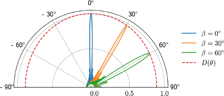
Figure 1.9. Radiation patterns of a linear antenna composed of 64 elements of width 2d = 4 mm and height 2h = 4 cm at a frequency f = 100 kHz. For a color version of this figure, see www.iste.co.uk/royer/waves2.zip
Its maximum value (2N) is divided by ![]() when α = ±0.885π/2, that is:
when α = ±0.885π/2, that is:
i.e. Δθ ≈ 3◦ for L = 256 mm and λ = 15 mm.
Figure 1.10 is an example of the measurement of the dispersion curves of a 1-mm thick duralumin plate using a linear array composed of 128 rectangular elements of dimensions 0.2 ×10 mm2 and spaced apart by 0.25 mm. A film of water ensures the coupling between the probe and the sample. A programmable electronic device transmits pulses to the first element, of center frequency 8 MHz and duration 4 μs, whose spectrum ranges from 4 to 12 MHz. This electronic device records the 128 signals received by all the elements. The Fourier transforms with respect to the time and space of these signals, acquired over 25 μs, are stored in a matrix. The N non-zero components are stored in a N × 3 (kn, fn, wn) matrix, where k, f and w represent, respectively, the wave number, frequency and Fourier coefficient. The representation in the “frequency-wave number” plane reveals the Lamb modes, characteristic of the propagation in a plate (section 4.3.1.2 in Volume 1). As noted in section 4.3.2 of Volume 1, the coupling with water does little modify the phase velocity of Lamb modes (Bochud et al. 2018).

Figure 1.10. Experimental dispersion curves of Lamb waves propagating in a duralumin plate of thickness 1 mm, measured using an array of 128 rectangular elements. For a color version of this figure, see www.iste.co.uk/royer/waves2.zip
1.1.5. Impulse diffraction
In domains like medical ultrasound imaging or non-destructive testing of materials, transducers that generate acoustic waves are often excited by short pulses. The velocity potential at point M and angular frequency ω is obtained by replacing the wave number k by ω/c in the expression [1.25] for the Rayleigh integral, established in the harmonic case:
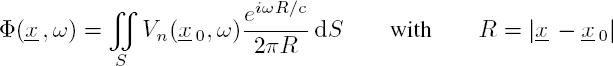
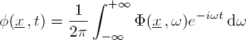
Φ(x, ω) is the spectral component, at angular frequency ω, of the instantaneous potential φ(x, t) at the observation point M. Similarly, Vn(x0, ω) is the spectral component of the normal velocity vn(x0, t) at point P on the emitting surface. The inverse Fourier transform:
is written as given below, by changing the integration order:
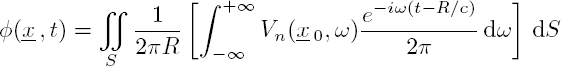
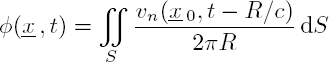
The integral in square brackets represents the normal component of the particle velocity at point P and time t – R/c, that is, vn(x0, t – R/c). Thus, the Rayleigh integral can be expressed in the time domain by:
1.1.5.1. Piston mode
Let us consider the case where all points of the source vibrate with the same normal velocity v0(t):
where Pn(x0) is the spatial amplitude profile of the vibration over the piston. Since the Dirac delta function δ(t) is the neutral element of the convolution operator, the function v0(t − R/c) can be written as:

By substituting equations [1.72] and [1.73] into relation [1.71], we get:

with:
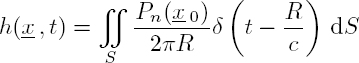
The velocity potential at point M is the convolution product of the velocity v0(t) at the piston surface with the space-time function h(x, t), called the diffraction impulse response at point M and time t. This result expresses the linearity and time invariance of the model (Fink and Cardoso 1984). This concept of an impulse response, that is, the response to a pulse shorter than the smallest characteristic time of the system, is commonly used in signal processing.
The Fourier transform of a convolution product is the simple product of transforms:
the diffraction frequency response H(x, ω) being the Fourier transform of h(x, t):

1.1.5.2. Plane uniform transducer
To calculate the diffraction impulse response of a plane transducer vibrating uniformly: Pn(x0) = 1, one approach is to note that in the integral [1.75], due to the term δ(t – R/c), only source points located at a distance R = ct contribute to the field at point M and time t (Figure 1.11). These points are located on a circular arc, centered at the projection M0 of the observation point M onto the plane of the disk. The radius ρ of this arc is such that:

The surface element is dS = L(R) dρ where L(R) is the length of the circular arc. Since δ(t – R/c) = cδ(R – ct), the impulse response [1.75] takes the form Stepanishen (1971):
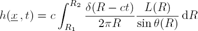
where R1 = ct1 and R2 = ct2 denote, respectively, the minimum and maximum distances from the points on the disk to the observation point M. The integration amounts to replace R with ct:
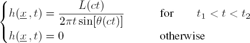
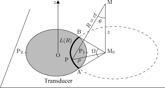
Figure 1.11. At time t, the contribution to the acoustic field at point M comes from the source points on the circular arc AB, where the transducer plane intersects the sphere of radius R = ct centered at M
An even simpler expression is obtained by introducing the angle Ω(R = ct) which, from its center M0 (Figure 1.11), subtends the circular arc AB of length:
The impulse response [1.80] takes the equivalent form:

In the case of the uniform disk of radius a, the field only depends on the variables r, z and t. For points located on the piston axis (r = 0) and for time t such that:
the arcs that are equidistant from the observation point are complete circles, therefore Ω(ct) =2π:
Since it is zero at other instants, the diffraction impulse response is a rectangular function whose duration:
decreases as the distance z increases (Figure 1.12).

Figure 1.12. Uniform disk of radius a. For a point M located on the z axis (a), the diffraction impulse response (b) is a rectangle of height c between times t1 = z/c and 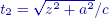
The acoustic pressure radiated by a circular disk, animated by a velocity v0(t), can be deduced from the time derivative of the velocity potential (equation [1.4]), that is, considering the convolution product:

On the piston axis, the derivative of the impulse response (Figure 1.12(b)) consists of a positive delta at time t1 and a negative delta at time t2; we obtain:
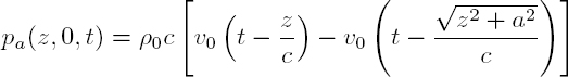
Figure 1.13(a) shows that in the vicinity of the disk (z << a), the acoustic pressure is formed of a first term similar to the surface velocity (plane wave) and a second term, of opposite sign, whose arrival time corresponds to a path coming from the edge of the disk. This edge wave expresses the diffraction effects related to the finite radius a of the source. At a larger distance (z = 2a), the two waves begin to overlap (Figure 1.13(b)). The interference phenomena, which are responsible for the oscillations of the acoustic pressure observed on the piston axis in the sinusoidal case (Figure 1.4), disappear in the impulse regime, because the acoustic field received at one point and at a given time arises from a well-defined area on the surface of the transducer.
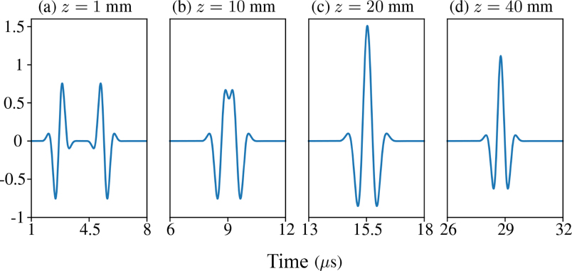
Figure 1.13. Acoustic pressure emitted (in water) on the z axis of a plane transducer, of radius a = 5 mm and central frequency 1 MHz, excited by a short pulse. In the far field (d), the pressure is similar to the derivative of the velocity on the surface of the disk
When the Fresnel approximation is valid, the duration Θ of the impulse response is inversely proportional to the distance z:
When z2 >> a2, the diffraction frequency response H(x, ω), that is, the Fourier transform of h(x, t), undergoes a dilatation along the frequency axis, proportional to z.
In the far field (Fraunhofer zone), the diffraction impulse response tends toward a Dirac pulse, that is, considering the unit area of the Dirac delta function:
The velocity potential is similar to the velocity v0(t) of the points on the surface of the piston disk (formula [1.74]):

and the acoustic pressure:
is similar to the derivative of the surface velocity of the disk (Figure 1.13(d)).
Figure 1.14 shows that the acoustic pressure passes through a maximum at a distance such that the opposite contributions of plane wave and edge wave (equation [1.87]) are added, that is, when their path difference is equal to half a wavelength:

This “pseudo-focusing” distance corresponds to the position, z1, of the last maximum (equation [1.41]), that is, the limit between the near field and the far field in the harmonic case.
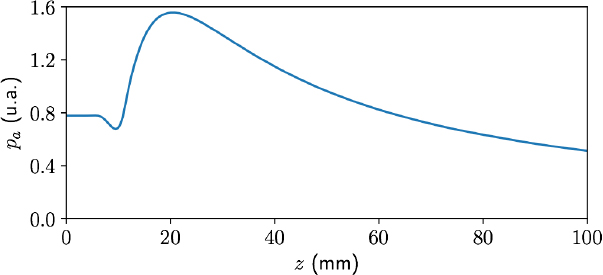
Figure 1.14. Maximum of the acoustic pressure emitted in pulse regime by a plane transducer of radius a = 5 mm, and central frequency 1 MHz versus the z position on its axis
REMARK.– The analysis of acoustic wave radiation by a transducer operating in the piston mode was conducted in two extreme cases, corresponding to the first two entries in Table 1.1:
- – in the harmonic case, that is, for a sinusoidally vibrating piston with a constant amplitude;
- – in the impulse regime, that is, for an infinitely short excitation (Dirac pulse).
We have shown that the radiated acoustic fields were very different (see, for example, Figures 1.4 and 1.14). In the ultrasonic domain, the need for a good axial resolution leads to the reduction of the time duration of the transmitted wave train. However, the center frequency and the bandwidth of the transducer impose a low limit on this duration (section 3.1.3). In practice, it varies from one period (very large bandwidth transducer) to a few tens of periods (narrow band transducer). The space-time evolution of the acoustic field, emitted in this transient regime, can then be calculated in two ways: either by summation of the contributions of the various spectral components (Fourier analysis) or, directly in the time domain, by convolution between the piston surface velocity and the diffraction impulse response.
1.1.5.3. Concave uniform transducer
In the far field, the acoustic beam emitted by a plane disk spreads due to diffraction: the acoustic intensity and lateral resolution decrease. A solution to improve these two parameters, essential to any imaging system, is to focus the acoustic beam either through a lens, like in optics, or by simply using a curved emitting surface.
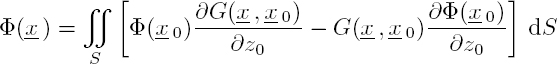
The geometry of a focused transducer whose surface is a spherical cup is defined by its radius of curvature or focal length F, and by the radius a of its circular edge (Figure 1.15(a)). The wave radiated into the fluid by a concave source can be diffracted by its own surface, giving rise to a secondary radiation. Strictly speaking, the Rayleigh integral no longer applies. However, this secondary diffraction is negligible if the curvature of the surface is slight (F >> a). In this case, the angle θn, between the normal to the emitting surface and the z axis, is small (θn ≤ arctan(a/F )). By equating the normal derivative ∂/∂n with the axial derivative ∂/∂z, expressions [1.75] and [1.77] for the Rayleigh integral are a good approximation of the radiated acoustic field.

Figure 1.15. Spherical cup, (a) focal length F, radius a, thickness e. (b) Calculation of the contribution to the radiated field at point M and time t
1.1.5.3.1. Diffraction impulse response
In the case of a uniform vibrating surface: Pn(x0) = 1, the velocity potential φ(x, t) and the diffraction impulse response h(x, t) are given by:

As for the plane disk, the surface element dS is equal to L(R) dζ, where L(R) is the length of the intersection of the spherical cup of radius F, with the sphere of radius R = ct centered at the observation point M (Figure 1.15(b)), and dζ is the width of the band intercepted on the spherical cup. The result obtained by Penttinen and Luukkala (1976) is:

where:
is the distance between the observation point M(z, r) and the focus F(F, 0). t1 and t2 are the extreme arrival times of the disturbance emitted, at time t = 0, by all the points on the transducer. Ω(ct) is the angle that subtends the arc formed by the points on the cup located at a distance R = ct from point M.
At any point on the axis (r = 0), since Ω(ct) = 2π and d(z, 0) = |F – z|, the diffraction impulse response takes the form of a rectangular function:

Denoting the thickness of the spherical cup by:
the minimum and maximum transit times are
for disturbances emitted by the center and the edge of the cup, respectively. It must be noted that if z < F, then t1 < t2 and, conversely, if z > F, then t1 > t2. Considering expression [1.4], the acoustic pressure created by a surface velocity v0δ(t) derives from the potential φ(t) = v0h(t):

that is, for its Fourier transform:

Given the value [1.98] of the limiting times t1 and t2 of the rectangle, the ratio of the acoustic intensity I(z) = |Pa(z)|2/2Z0 to the intensity I0 = Z0v2/2 on the transducer surface is given by:
Figure 1.16 represents the variations of the acoustic intensity I(z)/I0 normalized by the intensity I0 on the surface of a transducer of focal length F = 50 mm, radius a = 10 mm, that is, e = 1 mm, excited at a frequency f = 2.4 MHz, so that ke = 10. Before the focus, the oscillations resulting from the interference between waves emitted by the edge and the center of the cup are much smaller than in the case of a plane disk. The maximum of the relative intensity is located a little before the focus; beyond this point the acoustic intensity decreases rapidly with the distance.
When the observation point goes toward the focus (z → F ), the duration of the response tends to zero, while its amplitude tends to infinity. The diffraction impulse response converges to a Dirac function, whose intensity A is equal to the limit, when z approaches F, of the area of the rectangle of height cF/|F − z| and duration |t1 − t2|:
As to the first order in (z − F ):
the area A of the rectangle is equal to the thickness e of the spherical cup, so that:
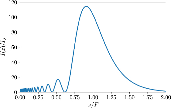
Figure 1.16. Normalized intensity along the axis of a transducer of focal length F = 50 mm and radius a = 10 mm
At the transducer focus, the velocity potential is a replica of the velocity v0(t) of the points on the emitting surface: φ(F, 0, t) = ev0(t – F/c). The velocity along z is proportional to the derivative of v0(t) delayed by F/c:

Beyond the focus, the shape of the velocity no longer changes and only its amplitude decreases due to the divergence of the beam. The particle velocity (or acoustic pressure) undergoes a time-derivative as it passes through the focus of the transducer.
As mentioned at the beginning of this section, the advantage of using a focused transducer is to achieve better performances in acoustic detection or ultrasonic imaging. In the following, we evaluate these improvements in terms of sensitivity and spatial resolution.
1.1.5.3.2. Acoustic intensity at the focus, diameter of the focal spot
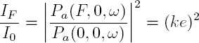
The acoustic pressure is given by relation [1.4] and the diffraction frequency response H(F, 0, ω) is the Fourier transform of the impulse response [1.104]:
Since, in the frequency domain Φ(F, 0, ω) = H(F, 0, ω)V0(ω), the modulus of the acoustic pressure at the transducer focus is equal to:
On the surface of the spherical cup, pa(0, 0, t) = ρ0cv0(t), hence Pa(0, 0, ω) = ρ0cV0(ω), and the ratio of the acoustic intensities is equal to the ratio of the square of the acoustic pressure moduli:
Assuming that a2 << F2, the thickness of the spherical cup can be written as e ≈ a2/2F and the gain in intensity:
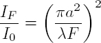
is larger than unity if the dimensionless parameter λF/a2 is less than π, that is, if the focal length F is smaller than the Rayleigh distance (Kino 1987), defined by:
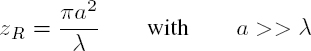
Energy concentration is only possible in the near field, beyond this limit the natural divergence of the acoustic beam prevails over the focusing effect due to the curvature of the spherical transducer.
In the piston mode, the mean power emitted by the entire surface of the transducer is πa2I0. By defining the diameter of the acoustic beam at the focus by the value 2w, such that half the emitted power passes through the interior of a circle of radius w, we obtain:

The width of the acoustic beam at –3 dB is thus written as:
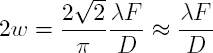
where D and F/D are, respectively, the diameter and the F-number of the transducer.
1.2. Generation of elastic waves by a surface source
In order to examine the radiation of bulk and surface elastic waves by sources distributed on the surface of a solid, we use Fourier analysis and the formalism of the mixed matrix, discussed in Appendix 2. The approach is as follows:
- – expression of stresses in the harmonic case as a function of the amplitudes of the rising and falling waves;
- – matrix inversion to calculate, using the emission matrix, the amplitudes of the emitted waves as functions of the forces applied on the solid surface;
- – calculation of the inverse Fourier transform to obtain the spatiotemporal response. In the near field, the inversion is carried out numerically; in the far field, approximate analytical expressions for the mechanical displacements at the arrival time of the bulk wave fronts and the Rayleigh wave fronts are obtained using the stationary phase method.
The method is applied to the case of an infinitely long and thin line source located along the x3 axis, on the surface of a solid occupying the half-space x2 > 0; the impulsive forces are either normal or parallel to the surface (Figure 1.17).
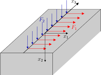
Figure 1.17. Arrangement of the line source on the surface x2 = 0 of the solid. The normal force density per unit length is F2. The tangential force density is F1. For a color version of this figure, see www.iste.co.uk/royer/waves2.zip
The mixed matrix M relates the amplitude a of the upward bulk waves and the amplitude b of the downward waves to the mechanical traction Tk = σk2 and the displacements ui on the solid surface. The physical meaning of the sub-matrices is given in Appendix 2. Here, in the absence of any rising wave (a= 0 ) and according to definition [A2.1], only the matrices E and Y come into play to express, in terms of the mechanical traction Tk, the amplitudes bJ of the emitted bulk waves and the components ui of the displacement on the free surface:
To arrive at a two-dimensional problem, the material, a priori anisotropic, is assumed to have an orthotropic symmetry with a binary axis parallel to x3. The propagation of QL and QT waves, polarized in the x1x2 plane, is then decoupled from the propagation of the TH wave, polarized along x3 (Volume 1, section 2.2.2.1). The slowness component s3 is equal to zero and the propagation direction in the sagittal plane is defined by the ratio m = s2/s1 of the two other components. By taking s1 as variable, the Christoffel equation is a fourth-degree polynomial equation in s2, whose coefficients are real. This admits four real or complex roots. Each real root corresponds to a propagative bulk wave transporting energy. The direction of the power flux is given by the normal to the slowness surface. The complex roots appear in conjugated pairs and only the two solutions decreasing with x2 must be retained as components of the Rayleigh wave. These two acceptable roots (s2J with J = 1,2) and all the elements of the mixed matrix are expressed as a function of a single variable: the slowness component s1.
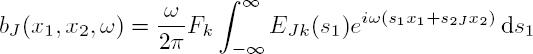
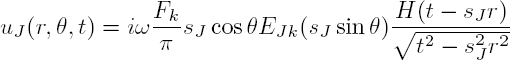
We first examine the generation of bulk waves polarized in the sagittal plane and then the generation of Rayleigh waves. In the harmonic case, an integral expression gives the mechanical displacement created in an elastic solid by a distribution of mechanical traction Tk(x1) exp(–iωt) applied to the free surface of the solid at x2 = 0. The relation [1.113] shows that the components EJk of the emission matrix are the coefficients of generation of the bulk elastic wave J by a tangential force (k = 1) or a normal force (k = 2). A surface excitation, concentrated along the x3 axis: Tk(x1) = Fkδ(x1) can be developed as the sum of spatial harmonics:

As the mechanical traction Tk = σk2 is expressed in N/m2, Fk is expressed in N/m: this is the force density per unit length along x3. In the plane of abscissa x2, the complex amplitude b J of the bulk wave J created by the uniform elementary force Fk dk1, parallel to the xk axis is:
By introducing, for the mode J, the components s1 = k1/ω and s2J = k2J /ω of the slowness vector, the total amplitude emitted by the line source is given by the integral:
1.2.1. Solid with orthotropic symmetry
We begin by developing the method in the general case of a medium with orthotropic symmetry, before applying it to an isotropic solid, and then to a material of cubic symmetry. The propagation equations for the QL and QT plane waves polarized in the x1x2 plane of an orthotropic solid were developed in sections 2.5.5 and 3.1.2.2 of Volume 1. With a mechanical displacement:
they are written in matrix form (Volume 1, system [3.43] with m = k2/k1):

Dividing by ω2 reveals the slownesses s1 = k1/ω and s2 = k2/ω. The characteristic equation:
is a biquadratic equation in ![]()
whose coefficients α0, α2 and α4 are given by relations [2.172] of Volume 1. The two acceptable roots (J = 1, 2) corresponding to the quasi-longitudinal wave (s21) and quasi-transverse wave (s22) depend on the slowness s1 through the intermediary of coefficients α2 and α0:

The polarization vector components for each wave, q1J and q2J, are related by:
where s2J (J = 1, 2) are the two positive roots of equations [1.121]. The stresses Ti = σi2 on the surface x2 = 0 are expressed using the coefficients BiJ (Appendix 2) and the amplitudes bJ of QL and QT waves:

The expressions for these coefficients, identical to those for coefficients AiJ, are given as functions of the parameter mJ = s2J /s1 by relations [2.150] in Volume 1, that is:

The inversion of the linear system [1.123], that is, of matrix B, provides the four components EJk of the emission matrix E, required for the calculation of the integral [1.116], giving the amplitude bJ of wave J created by the force density Fk:

Since the amplitudes of the partial waves, that is, the components of vector b, are obtained in the Fourier domain, the components of the displacement field in the real space are calculated by numerical inverse Fourier transforms. However, the presence of singularities associated with the poles or the branch points makes the inversion difficult. The introduction of a small imaginary part in the angular frequency allows us to move away from these singularities while keeping their significant influence (Weaver et al. 1996).
The generation of elastic waves by a line source in a duralumin half-space is illustrated in Figure 1.18. The source, located at (x1, x2) = (0, 0), is a very short impulse. Four types of waves are visible: the first two are longitudinal (L) and transverse (T) bulk waves, which propagate with a cylindrical wave front, diverging from the line source. Two Rayleigh (R) waves propagate on the free surface on both sides of the source. Finally, two head waves (H) can also be observed on either side of the source. These head waves are transverse waves resulting from the conversion of the grazing longitudinal wave beyond the critical angle θc = arcsin(VT /VL) (see Chapter 2 of Volume 1). Due to this conversion, the grazing longitudinal wave radiates energy toward the inside of the material, implying that it is attenuated during its propagation.
The generation of elastic waves by an impulse line source in a copper half-space is illustrated in Figure 1.19. The comparison of this map at time t = 40 μs with the wave surfaces in Figure 1.13(b) of Volume 1 clearly shows quasi-longitudinal and quasi-transverse wave fronts.
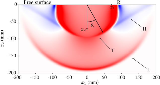
Figure 1.18. Isotropic solid. Map of the amplitude of the displacement generated by an impulse line source and wave fronts. For a color version of this figure, see www.iste.co.uk/royer/waves2.zip

Figure 1.19. Anisotropic solid. Map at time t = 40 μs after the application of an impulsive force, showing the amplitude of the displacement generated by a line source in a copper crystal with cubic symmetry. For a color version of this figure, see www.iste.co.uk/royer/waves2.zip
1.2.2. Far field
In this section, the integral [1.116] is evaluated by the stationary phase method. This approximation is valid in the far field and in the vicinity of the wave fronts of bulk waves, when they propagate independently. The directivity functions are plotted for an isotropic solid. In the case of an anisotropic material, the focusing effect due to the variations in curvature of the slowness surface is highlighted. Then, we calculate the contribution of the Rayleigh wave to the mechanical displacement of the solid surface.
1.2.2.1. Bulk waves: directivity diagrams
When k1x1 is very large compared to unity, the phase variations:
cause very rapid oscillations (as functions of s1) of the exponential eiϕ(s1), which contribute little to the integral [1.116]. The major part of its value comes from the interval around the slowness ![]() where the phase ϕ(s1) is stationary, that is, for which the derivative dϕ/ds1 cancels. The second-order development is a good approximation of the phase in the vicinity of
where the phase ϕ(s1) is stationary, that is, for which the derivative dϕ/ds1 cancels. The second-order development is a good approximation of the phase in the vicinity of ![]()

Let us carry over this development into [1.116] and by assuming that the variations in factor EJk(s1) are slow compared to the variations in the exponential, we get:

By changing the variable:
and since ![]() we obtain:
we obtain:
As:

the amplitude of the wave J emitted by the source is given by equation [1.116]:
1.2.2.1.1. Isotropic solid
As s1 = sJ sin θ and s2 = sJ cos θ, at the fixed observation point M(x1, x2), the derivative of the phase:

vanishes for the angle θ0, so that tan θ0 = x1/x2 and the second derivative is negative:

By introducing the wave number kJ = ωsJ, we get:
With ε = −1, equation [1.132] gives the amplitude of the longitudinal (J = 1) and transverse (J = 2) displacements generated by a linear distribution of tangential (k = 1) or normal (k = 2) forces:

This amplitude decreases in ![]() as expected for cylindrical waves emitted by a line source. The last term of the right member is, in the two-dimensional case, the far field approximation of the spectral Green’s function of the Helmholtz equation:
as expected for cylindrical waves emitted by a line source. The last term of the right member is, in the two-dimensional case, the far field approximation of the spectral Green’s function of the Helmholtz equation:
Taking into account its asymptotic behavior, the zero-order Hankel function of first kind ![]() is the appropriate solution for a divergent wave and a temporal factor in e−iωt:
is the appropriate solution for a divergent wave and a temporal factor in e−iωt:

Given the expression for the time Green’s function, that is, the Fourier transform of G(r, ω):

where H(t) is the unit step (Heaviside) function, the instantaneous displacement is given by:
Normal force (k = 2)
The coefficients E12(s1) and E22(s1) are calculated in Appendix 2:

where Δ(s1) is the Rayleigh determinant:
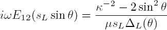
- – In the case of a longitudinal wave: s1 = sL sin θ and s2L = sL cos θ, the Rayleigh determinant is expressed by:
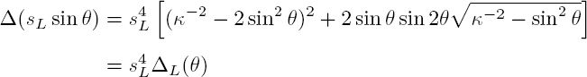
with κ = sL/sT. By replacing s1 by sL sin θ in the numerator of E12, we get:
and the displacement in the far field [1.140] is equal to:
D2L(θ) is the dimensionless directivity factor for a normal force:

- – In the case of a transverse wave s1 = sT sin θ and s2T = sT cos θ, the Rayleigh determinant is expressed by:

By replacing s1 by sT sin θ in the numerator of E22, we obtain:
The transverse displacement in the far field is given by expression [1.145], by replacing D2L(θ) with:

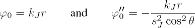
The directivity patterns D2L(θ) and D2T (θ) are plotted in Figure 1.20 in the case of duralumin (κ = VT /VL = 0.5) and for a material of Poisson’s ratio ν = 0.2. The radiation of the longitudinal wave is maximum at the center. The source is omnidirectional but not isotropic. For transverse waves, the source is more directional. Maximum energy is radiated at an angle close to 35◦.

Figure 1.20. Normal force. Radiation patterns for a line source: a) longitudinal wave; b) transverse wave for two values of the Poisson’s ratio: ν = 0.2 and ν = 1/3. For a color version of this figure, see www.iste.co.uk/royer/waves2.zip
ORDER OF MAGNITUDE.– The amplitude of the mechanical displacement, proportional to the ratio of the force density F2 (N/m) to the shear modulus μ (N/m2), is expressed in meters. In the ultrasound domain, the displacements are of the order of a few nanometers. For example, with constants close to those of duralumin: μ = 25 GPa, κ = 0.5 and F2 =1 N/cm, we obtain D2L(0) = κ2 = 0.25 and uL =1 nm.
Tangential force (k = 1)
The elements E11(s1) and E21(s1) of the emission matrix [A2.24] are:

and the Rayleigh determinant is still expressed by:
Replacing s1 by sL sin θ in the numerator of E11, the longitudinal displacement created in the far field by the tangential force distribution of density F1 is given by:

where the directivity factor D1L(θ) has the same denominator as D2L(θ):
Similarly, by replacing s1 by sT sin θ in E21, the transverse displacement is given by expression [1.152] by changing D1L(θ) in:

The denominator of D1T(θ) is identical to that of D2T(θ).
Figure 1.21(a) shows that there is no radiation in the form of a longitudinal wave along the normal to the surface. The emission is maximum in a direction depending on the ratio κ = VT /VL, which is close to 65◦ in the case of duralumin (ν ≈ 1/3). For transverse waves (Figure 1.21(b)), maximum energy is radiated at an angle close to 30◦. Emission is always zero for θ = 45◦ due to the cancellation of the term cos 2θ in formula [1.154]. The main and secondary lobes have opposite polarities.
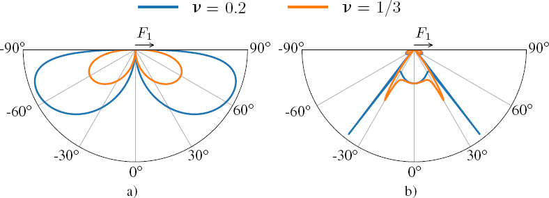
Figure 1.21. Tangential force. Radiation patterns for a line source: a) longitudinal wave; b) transverse wave for two values of Poisson’s ratio: ν = 0.2 and ν = 1/3. For a color version of this figure, see www.iste.co.uk/royer/waves2.zip
Since the ratio κ−2 = (VL/VT )2 is greater than 2 for any isotropic solid, the directivity functions D1L and D2L are real for any θ. On the other hand, the functions D1T and D2T are real for θ smaller than the critical angle θc = arcsin(VT /VL) and complex for θ > θc.
1.2.2.1.2. Anisotropic solid
The energy velocity vector V e is at all points normal to the slowness surface: V e. ds= 0. Assuming that the sagittal plane is a symmetry plane, V e is contained in this plane and the angle θe of the acoustic ray, with respect to the normal x2, is given by tan θe = ds2/ ds1. For a given source–receiver configuration, the derivative of the phase:

vanishes if tan θe = x1/x2. Consequently, the value ![]() for which the phase is stationary is such that the acoustic ray is parallel to the direction joining the emission point O to the observation point M (Figure 1.22).
for which the phase is stationary is such that the acoustic ray is parallel to the direction joining the emission point O to the observation point M (Figure 1.22).
The associated point L on the slowness curve of mode J defines the propagation angle θ through:
Setting OM = r: x1 = r sin θe, x2 = r cos θe, the value of the phase ![]() is:
is:
where ψ = θe − θ is the deviation angle between the energy velocity vector and the propagation direction. Let us calculate the second derivative from the expression [1.155] of the first derivative:
By using the relation ds/dθ = –s tan ψ (Figure 1.22) to evaluate the derivative of s1 = s(θ) sin θ, we obtain:

Figure 1.22. Bulk wave generation in an anisotropic medium. Position of the stationary phase point L on the slowness curve, corresponding to the observation point M
By introducing the wave number ![]() corresponding to the energy velocity
corresponding to the energy velocity ![]() we get:
we get:

The amplitude of the wave J transmitted in the direction θ is given by [1.132]:
The phase ![]() is proportional to the time
is proportional to the time ![]() taken by the energy to reach the observation point distant from r. This result agrees with the fact that in a point source and point receiver configuration, the mechanical disturbance propagates at the energy velocity in the source–receiver direction.
taken by the energy to reach the observation point distant from r. This result agrees with the fact that in a point source and point receiver configuration, the mechanical disturbance propagates at the energy velocity in the source–receiver direction.
In addition to the product sJ (θ) cos θe, the angular dependence of the amplitude comes from the emission coefficient EJk(sJ sin θ) and from the term A = |dθ/dθe||. This focusing factor, postulated by Maris (1971) in order to explain the phonon focusing observed in crystals, measures the anisotropy of the ray density, that is, the concentration of acoustic energy. For the displacement amplitude, the relevant quantity is ![]() In highly anisotropic materials such as carbon-epoxy composites, this focusing effect dominates the variation with respect to the propagation direction of the emission coefficient (Corbel et al. 1993). Strong focusing (A >> 1) occurs when the direction of the energy velocity remains the same while the propagation direction varies (|dθe/dθ| << 1). Let us note that the stationary phase approximation breaks down for directions such that dθe/dθ = 0, for which
In highly anisotropic materials such as carbon-epoxy composites, this focusing effect dominates the variation with respect to the propagation direction of the emission coefficient (Corbel et al. 1993). Strong focusing (A >> 1) occurs when the direction of the energy velocity remains the same while the propagation direction varies (|dθe/dθ| << 1). Let us note that the stationary phase approximation breaks down for directions such that dθe/dθ = 0, for which ![]() The existence of a singularity for the displacement amplitude corresponds to points at which the curvature of the slowness curve vanishes, for example, in the presence of caustics. The ray model also becomes inaccurate when the emission factor EJk(s1) is canceled for, or in the vicinity of, the value
The existence of a singularity for the displacement amplitude corresponds to points at which the curvature of the slowness curve vanishes, for example, in the presence of caustics. The ray model also becomes inaccurate when the emission factor EJk(s1) is canceled for, or in the vicinity of, the value ![]()
Therefore, the exact calculation of the dynamic response of an anisotropic solid half-space to a local and transient solicitation is complex. An analytical solution consists of determining the Green’s function G(s1, x2, p) in the space of the Laplace transform for time (complex variable p) and in the space of the Fourier transform according to x1 (complex variable k1 = –ips1). The inversion of these transforms in order to calculate the impulse response g(x1, x2, t), for example, by using the Cagniard-De Hoop method, requires rigorous mathematical developments (Poncelet and Deschamps 2009).
1.2.2.2. Rayleigh wave
On the surface of an elastic solid, the disturbance arising from a line source is composed of a part corresponding to the head wave and of a part corresponding to the Rayleigh wave (Figure 1.18). Unlike the head wave, the amplitude of the Rayleigh wave does not decrease during propagation. Then, far from the source, the Rayleigh wave predominates.
Relation [1.113], namely ui = YijTj, shows that the components Yij of the admittance matrix Y are the generation coefficients of the displacements in the plane of the surface (i = 1) or out-of-plane (i = 2), produced by a uniform distribution of tangential mechanical traction (j = 1) or normal mechanical traction (j = 2), applied on the free surface of an elastic solid. These coefficients only depend on the slowness component s1 = k1/ω. The displacement generated by a spatially varying force Tj(x1) is obtained by Fourier analysis:
where ![]() is the Fourier transform of the spatial distribution Tj(x1). If the force is concentrated on the surface, along the line
is the Fourier transform of the spatial distribution Tj(x1). If the force is concentrated on the surface, along the line ![]() Fj. The mechanical displacement is expressed as:
Fj. The mechanical displacement is expressed as:

is the spectral Green’s function. The integral only depends on a single variable: the product ωx1. For an isotropic solid, the Yij components take the form (Appendix 2):

where Δ(s1) is the Rayleigh determinant. The normal slownesses s2L and s2T are imaginary:
so that the displacements of the Rayleigh wave ![]() decrease with depth x2 > 0 in the material. The Rayleigh determinant [1.142] is written as:
decrease with depth x2 > 0 in the material. The Rayleigh determinant [1.142] is written as:
Each solution s1 = ±sR with sR > sT > sL to the Rayleigh equation Δ(s1) = 0 corresponds to a pole of all admittance coefficients Yij. The contribution from these poles to the integral [1.163] provides the Green’s function ![]() for the surface displacement of the Rayleigh wave. This contribution is calculated by the residue method (Figure 1.23). The integration contour is closed by a semicircle C+ (C−) at infinity in the upper (lower) s1 half-plane when x1 is positive (negative), so that the factor
for the surface displacement of the Rayleigh wave. This contribution is calculated by the residue method (Figure 1.23). The integration contour is closed by a semicircle C+ (C−) at infinity in the upper (lower) s1 half-plane when x1 is positive (negative), so that the factor ![]() is zero on each semicircle.
is zero on each semicircle.
The poles ±sR are located on the integration contour because we have neglected the attenuation. To take this effect into account, we must associate a positive imaginary part with the pole +sR, corresponding to the propagation in the positive x1 direction (sR → sR + iα), so that the factor e−ωαx1 is canceled when x1 → +∞. Equivalently, a negative imaginary part must be associated with the pole −sR corresponding to the propagation in the negative x1 direction (−sR → −sR − iα). The contribution of the positive pole (integrating anticlockwise around C+) is given by:

that is:
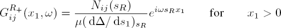

Figure 1.23. Integration contour in the complex plane to evaluate the contribution of poles ±sR. In the upper half-plane (Im[s1] > 0), the factor exp(iωs1x1) approaches zero when the radius of the semicircle C+ tends to infinity
Using the property which states that ( dΔ/ ds1) is an odd function s1, the contribution of the negative pole (integrating clockwise around C−) is:

The components of the matrix N (formulae [A2.27] in Appendix 2) are equal to:
and:

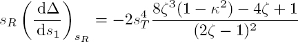
The sign of the displacement depends on the parity of the numerator. Since N22 (N21) is even (odd), a normal (tangential) force creates an equal (opposite) normal displacement moving off the source. The calculation (which is quite long) of the derivative of the Rayleigh determinant Δ(s1) for s1 = sR leads to an expression that depends on the parameters ![]()
Substituting the expressions for N12 and N22 in equation [1.168] provides the surface displacements (u1 and u2) of the Rayleigh wave generated by a line source of normal force density F2 (Lamb 1904; Achenbach 1987). Similarly, substituting N11 and N21 provides the Rayleigh wave displacements (u1 and u2) generated by a line source of tangential force density F1; for example, for x1 > 0:
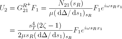
Considering [1.172], the normal displacement is given by:

REMARK.–
- – For x1 > 0, the displacement u2 is negative, because a positive tangential force F1 compresses the material; in the (x1 < 0) region, the same force creates a depression at the level of the free surface and u2 is positive.
- – The ratio of amplitudes b21/b11 = N21(sR)/N11(sR) is equal to that of transverse and longitudinal components of the Rayleigh wave (relation [3.23] in Volume 1): the disturbance propagates on the surface without deforming it.
- – N21 is real, N11 is imaginary: the two displacement components are in phase quadrature.
ORDER OF MAGNITUDE.– For duralumin, ζ = 1.145 and κ = 0.486, hence R = 0.384; with μ ≈ 25 GPa, the amplitude of the normal displacement of the Rayleigh wave created by a linear tangential force, of density F1 = 1 N/cm, is b21F1 = 0.38 nm.
The time displacement, that is, the Fourier transform of U2(x1, ω):

is a Dirac function:
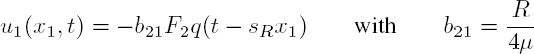
The mechanical displacement generated by a distribution of impulsive forces F1q(t) is obtained through the convolution with q(t):
It has the same time-dependence q(t) as the force that created it, while the temporal form of the tangential component is the Hilbert transform of q(t) (Royer 2001).
In the case of a normal force of density F2, since N12(sR) = −N21(sR), the expression for the tangential component ![]() is deduced from equation [1.173], by changing the sign and by replacing F1 by F2. The tangential displacement reproduces the time variation q(t) of the normal force:
is deduced from equation [1.173], by changing the sign and by replacing F1 by F2. The tangential displacement reproduces the time variation q(t) of the normal force:
Then, it is the normal component which is the Hilbert transform of q(t).
1.2.3. Generation in a plate
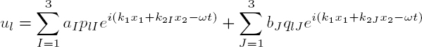
In practice, the propagation medium has finite dimensions. Let us study the generation in a plate, of thickness d, by a line source of normal forces. The observation point is located on the same side of the plate at a distance ℓ from the source. Assuming a Gaussian spatial distribution, uniform along x3, of width a along x1, the force density is of the form:

The function q(t) is normalized to unity and its duration at half-height is Δt ≈ 2.4τ. The width at −3 dB of its frequency spectrum Q(ω) is Δf ≈ 0.1/τ (Figure 1.24):

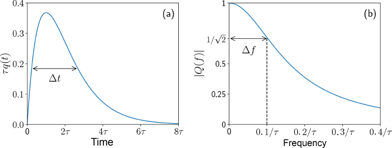
Figure 1.24. Function q(t) and modulus of its spectrum Q(f). a) The pulse duration Δt is equal to 2.4τ; b) the width Δf of its spectrum is about 0.1/τ
Compared to the case of a semi-infinite medium (section 1.2.1), the model takes into account all the upward waves (of amplitude aI) and downward waves (of amplitude bJ ). The expression [1.117] for the mechanical displacement is replaced by:
The normal components of the wave vector (k2I , k2J ) and the polarizations (plI , qlJ ) are determined by solving the Christoffel equation. The amplitudes (aI , bJ ) of the partial waves are deduced from the boundary conditions on the two free surfaces of the plate. In the case of an isotropic solid, the sums are limited to two terms, with I, J = 1 or 2 for longitudinal or transverse waves, respectively.
Figure 1.25 shows the mechanical displacement generated in a stainless steel plate of thickness d = 4 mm, for τ = 10 ns and a force F = 10−2 N, that is, F/a = 100 N/m, when a = 0.1 mm. The tangential component u1 and normal component u2 were calculated at a distance ℓ = 6 mm on the same face as the source. For both components, the first signal H corresponds to the head wave that propagates on the surface at a velocity VL = 5 634 m/s. The largest displacement R is that of the Rayleigh wave that propagates at the velocity VR = 3 015 m/s. The tangential component of the Rayleigh wave (Figure 1.25(a)) reproduces the time variation q(t) of the force while the normal component (Figure 1.25(b)) is similar to the Hilbert transform of q(t).
With a period τ = 10 ns, that is, Δf = 10 MHz, and for a frequency f = 5 MHz, the wavelength λR = VR/ f 0.6 mm is much smaller than the plate thickness. The Rayleigh wave propagates as if the medium were semi-infinite, ignoring the second face that is at a distance greater than 2λR.

Figure 1.25. a) Tangential displacement u1 and b) normal displacement u2, created by a line of normal forces in a 4-mm thick steel plate. The observation point is located on the same face, at a distance ℓ = 6 mm from the source
The other echoes are due to the successive reflections with the possible conversion of bulk waves on each free surface (section 2.4.1, Volume 1). For example, the echo 1T1L corresponds to a transverse wave on the forward path and a longitudinal wave on the return path converted during the reflection on the opposite face (Figure 1.26). Their arrival times are predicted by a ray model, using the relation:

where integers n and m, whose sum is necessarily even, correspond to the number of single paths from one face to another for L and T waves, between the line source and the receiver. For equal times of flight (for example, when n = m: tnT nL = tnLnT ), only one of these paths is shown in Figure 1.25.

Figure 1.26. Generation in a plate by a normal force. First echoes received at the point x1 = ℓ
The angles of incidence θL and θT, with respect to the normal to the plate, depend on the number of single paths for each wave. The projection of these paths on the x1 axis is:
Since angles θL and θT are related by the Snell–Descartes law sin θT = κ sin θL, equation [1.183] has only one unknown, for example, sin θL. Once the angles of incidence are determined, the arrival time tnLmT can be calculated using formula [1.182]. In Figure 1.25, the first echoes are indicated at their arrival times.
The echo H2T is different: it arises from the radiation of the head wave into a transverse wave at the critical angle θL = arcsin(κ). This wave is then reflected off the rear face of the plate, before reaching the receiver. The transit time associated with this path is given by:

Due to the energy loss through radiation toward the core of the plate, the head wave H and the echo H2T are rapidly attenuated when the distance ℓ increases.
In the case of a thin plate, whose thickness d is no longer large with respect to the wavelengths λR, λT and λL, the different echoes are superimposed. Far from the source, the successive reflections of L and T waves give rise to eigenmodes guided by the plate. For example, when d is of the order of λR, the coupling (symmetrical or antisymmetrical) of the Rayleigh waves propagating on both faces of the plate is at the origin of the two fundamental modes S0 and A0. These Lamb waves, studied in section 4.3.1 in Volume 1, are composed of both longitudinal and transverse vertical displacements. The proportion of these components and, thus, the phase velocity of Lamb waves vary with frequency.
1.3. Radiation of elementary spherical sources
In this section, we calculate the mechanical displacement radiated in an isotropic medium by a moving sphere. This sphere can expand and contract along its radius, or oscillate in a rotational or translational motion.
Let Rs be the reference frame with spherical coordinates (r, θ, ϕ) and center O. The Cartesian coordinates are then defined in terms of spherical coordinates through relations [A1.21]. The displacement field u, which is a solution to the propagation equation, is searched using the Helmholtz decomposition:
with:

where φL, φT and φS are scalar potentials, solutions to the Helmholtz equations:
By assuming that the motions are independent of the angle ϕ, the components of the displacement field are expressed in spherical coordinates as:

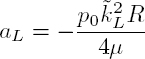
1.3.1. Pulsating sphere
Let us consider a sphere of radius R animated by a purely radial displacement (pulsating sphere). When the three potentials φL, φT and φS do not depend on the angle θ, only the radial displacement is non-zero; it derives from the scalar potential φL associated with the longitudinal wave:
This is the solution to the equation:
hence:

The first term represents a divergent wave, the second one a convergent wave, with amplitudes aL and bL. In the surrounding medium (r > R), the radial displacement ur and radial stress σrr of the divergent wave are written as (formula [A1.17] in Volume 1):

In the following, two cases are examined. If the sphere is animated by a radial displacement of amplitude U, the continuity of the displacement ur(R) = U leads to the following expression for the amplitude:
or again, if ![]()
If the sphere is a cavity with a pressure p0 that is assumed to be uniform on its surface, the continuity of the radial stress σrr(R) = –p0 allows us to express the amplitude aL through the relation:
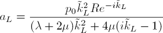
or again, if ![]()
1.3.2. Oscillating sphere with a rotational motion
Let there be a sphere animated by a rotational motion around the z axis, of angular amplitude Ω:
Since the movement of the sphere is, on the one hand, independent of the angle ϕ and, on the other hand, only polarized along the eφ axis, the wave excited by the rotation of the sphere derives only from the potential ϕS:
The displacement of the sphere imposes the following form for the potential ϕS:
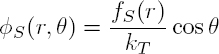
where the function fS satisfies the Helmholtz equation [A1.22]:
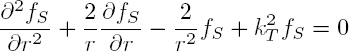
The solution is a linear combination of first-order spherical Hankel functions of the first and second kinds, ![]() that is:
that is:
These functions are associated with divergent and convergent waves. Only the divergent wave is generated by the motion of the sphere. With bS = 0, the displacement is given by:
The continuity of the displacement uφ on the surface of the sphere [1.197] imposes:

At low frequency and in the far field (kT r >> 1 and ![]() the displacement is given by:
the displacement is given by:
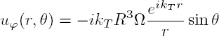
1.3.3. Oscillating sphere with a translational motion
Let there be a sphere animated by a translational motion of amplitude U along the z axis. In the reference frame with spherical coordinates, the displacement components at each point on the sphere are expressed by:
Since the motion of the sphere is independent of the angle φ and is contained in the (er, eθ) plane, the wave emitted by the sphere is described by potentials ϕL and ϕT of the type:
The functions fM (r) are the solutions to equation [1.200]. Retaining only terms that correspond to divergent waves, they take the form:
and the non-zero components of the displacement are given by:
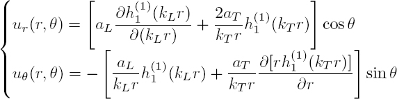
Considering expression [A1.39], the application of the boundary conditions at r = R leads to the following relations, by writing ![]()
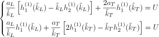
The resolution of these equations leads to the expressions:

that is, when the longitudinal and transverse wavelengths are large compared to the radius R of the sphere (![]() M << 1):
M << 1):
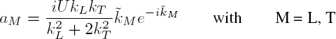
Given the limit of the function ![]() for large arguments (formula [A1.40]), the approximate expressions for the displacement components in the far field are:
for large arguments (formula [A1.40]), the approximate expressions for the displacement components in the far field are:

The mechanical displacement is calculated in the far field for a bead buried in an epoxy matrix. The components ur and uθ, associated, respectively, with the longitudinal and transverse waves, are plotted as functions of the angle θ in Figure 1.27 for the case of a sphere whose radius is (a) small compared to the wavelength, and (b) large compared to the wavelength. These diagrams depict the directivity of the mechanical displacement. For a sphere radius small compared to the wavelength, the radiation of the transverse wave is more intense than that of the longitudinal wave, while they are comparable for a sphere radius larger than the wavelengths. In both cases, the oscillation of the sphere in the z direction leads to the radiation of a longitudinal wave in this direction and of a transverse wave in the xy plane: the sphere motion imposes the polarization of the emitted waves.

Figure 1.27. Sphere embedded in an epoxy resin and oscillating in translation along the z axis. Components ur and uθ of the mechanical displacement as functions of the angle θ when a) λ >> R and b) λ << R. For a color version of this figure, see www.iste.co.uk/royer/waves2.zip
- 1 In the following and to simplify the notations, the reference to the angular frequency ω is removed for all quantities.
- 2 On the surface S, the outgoing unit normal is −ez, imposing a change of sign between equations [1.15] and [1.16].