
CHAPTER 35
Introducing Power Pivot
Recognizing the importance of the business intelligence (BI) revolution and the place Excel holds within it, Microsoft has made substantial investments in improving Excel's BI capabilities, specifically focusing on Excel's self-service BI capabilities and its ability to manage and analyze information better from the increasing number of available data sources.
The key product of this endeavor is Power Pivot. With Power Pivot comes the ability to set up relationships between large, disparate data sources and to merge data sources with hundreds of thousands of rows into one analytical engine within Excel.
Starting with the release of Excel 2013, Microsoft has incorporated Power Pivot directly into Excel. This means the powerful capabilities of Power Pivot are available to you right out of the box!
In this chapter, you'll get an overview of those capabilities, exploring the key features, benefits, and capabilities of Power Pivot.
Understanding the Power Pivot Internal Data Model
At its core, Power Pivot is essentially a SQL Server Analysis Services engine made available through an in-memory process that runs directly within Excel. The technical name for this engine is the xVelocity analytics engine. However, in Excel, it's referred to as the internal data model.
Every Excel workbook contains an internal data model, which is a single instance of the Power Pivot in-memory engine. This section outlines how to leverage the Power Pivot internal data model to import and integrate disparate data sources.
Activating the Power Pivot Ribbon
The Power Pivot Ribbon interface is available only when you activate it. It's important to note that the Power Pivot add-in does not install with every edition of Office. For example, if you have the Office Home edition, you will not be able to see or activate the Power Pivot add-in; thus, you will not have access to the Power Pivot Ribbon interface.
As of this writing, the Power Pivot Ribbon interface is available to you only if you have one of the following editions of Office or Excel:
- Office 2013, 2016, or 2019 Professional Plus: Available through volume licensing only
- Office 365 Pro Plus: Available with an ongoing subscription to
Office365.com - Excel 2013, 2016, or 2019 stand-alone edition: Available for purchase through any retailer
If you have any of these editions, you can activate the Power Pivot Ribbon by following these steps:
- Open Excel and look for a Power Pivot tab on the Ribbon. If you see the tab, then you can skip the remaining steps.
- On the Excel Ribbon, click File ⇨ Options.
- Choose the Customize Ribbon option on the left.
- Look in the Main Tabs list on the right and find the Power Pivot option. Check the box next to this option and click OK.
- The Power Pivot tab should appear (see Figure 35.1). If the Power Pivot tab does not appear in the Ribbon, close Excel and restart.

FIGURE 35.1 The Power Pivot Ribbon interface
Linking Excel tables to Power Pivot
The first step in using Power Pivot is to fill it with data. You can either import data from external data sources or link to Excel tables in your current workbook. For now, let's start this walk-through by linking three Excel tables to Power Pivot.
|
Most of the examples in this chapter are available on this book's website at |
In this scenario, we have three data sets in three different worksheets (see Figure 35.2): Customers, Invoice Header, and Invoice Details.

FIGURE 35.2 We want to use Power Pivot to analyze the data in the Customers, Invoice Header, and Invoice Details worksheets.
The Customers data set contains basic information like Customer ID, Customer Name, Address, and so forth. The Invoice Header data set contains data that points specific invoices to specific customers. The Invoice Details data set contains the specifics of each invoice.
We want to analyze revenue by customer and month. It's clear that we'll somehow need to join these three tables together before we can do our analysis. In the past, we would have to go through a series of gyrations involving VLOOKUPs or other clever formulas. But with Power Pivot, we can build these relationships in just a few clicks.
Preparing your Excel tables
When linking Excel data to Power Pivot, it's a best practice first to convert your Excel data to explicitly named tables. Although not technically necessary, giving your tables friendly names helps track and manage your data in the Power Pivot data model. If you don't convert your data to tables first, Excel will do it for you and give your tables useless names like Table1, Table2, and so on.
Follow these steps to convert each data set into an Excel table:
- Go to the Customers tab, and click anywhere inside the data range.
- Press Ctrl+T on your keyboard. This will activate the Create Table dialog box shown in Figure 35.3.

FIGURE 35.3 Convert your data range into an Excel table.
- In the Create Table dialog box, make sure the range for the table is correct and that the check box next to the “My table has headers” option is selected. Click the OK button.
- You should now see a Table Tools Design tab on the Ribbon. Click that tab and use the Table Name input to give your table a friendly name (see Figure 35.4). This will ensure that you will be able to recognize the table when adding it to the internal data model.

FIGURE 35.4 Give your newly created Excel table a friendly name.
- Repeat steps 1–4 for the Invoice Header and Invoice Details data sets.
Adding your Excel tables to the data model
Once you've converted your data to Excel tables, you're ready to add them to the Power Pivot data model. Follow these steps to add your newly created Excel tables to the data model using the Power Pivot tab:
- Click any cell inside your Customers Excel table.
- Click the Power Pivot tab on the Ribbon, and click the Add to Data Model command. Power Pivot creates a copy of your table and activates the Power Pivot window (shown in Figure 35.5).

FIGURE 35.5 The Power Pivot window shows all the data that currently exists in your data model.
Although the Power Pivot window looks like Excel, it's actually a separate program altogether. You'll notice that the grid for the Customers table has row numbers but no column references. You'll also notice that you can't edit the data within the table. This data is simply a snapshot of the actual Excel table you imported.
Additionally, if you look at your Windows taskbar at the bottom of your screen, you'll see that Power Pivot has a separate window from Excel. You can switch between Excel and the Power Pivot window by clicking each respective program in the taskbar.
Repeat steps 1 and 2 for your other Excel tables: Invoice Header and Invoice Details. Once you have imported all your Excel tables into the data model, your Power Pivot window will show each data set on its own tab, as shown in Figure 35.6.

FIGURE 35.6 Each table you add to the data model will be placed on its own tab in Power Pivot.
Creating relationships between your Power Pivot tables
At this point in our walk-through, Power Pivot knows that we have three tables in the data model, but it has no idea how these three tables relate to one another. We'll need to connect these tables by defining relationships between the Customers, Invoice Details, and Invoice Header tables. We can do so directly within the Power Pivot window.
- Activate the Power Pivot window, and click the Diagram View command button on the Home tab. Power Pivot will display a screen that shows a visual representation of all the tables in the data model (see Figure 35.7).

FIGURE 35.7 The Diagram view allows you to see all the tables in your data model.
You can move the tables in the Diagram view around simply by clicking and dragging their title bars. The idea is to identify the primary index keys in each table and connect them. In this scenario, the Customers table and the Invoice Header table can be connected using the CustomerID field. The Invoice Header and Invoice Details tables can be connected using the InvoiceNumber field.
- Click and drag a line from the CustomerID field in the Customers table to the CustomerID field in the Invoice Header table (as demonstrated in Figure 35.8).

FIGURE 35.8 To create a relationship, you simply click and drag a line between the fields in your tables.
- Click and drag a line from the InvoiceNumber field in the Invoice Header table to the InvoiceNumber field in the Invoice Details table.
At this point, your diagram will look similar to Figure 35.9. Notice that Power Pivot shows a line between the tables that you just connected. In database speak, these are referred to as joins.

FIGURE 35.9 When you create relationships, the Power Pivot diagram will show join lines between your tables.
The joins in Power Pivot are one-to-many joins. This means that when a table is joined to another, one of the tables has unique records with unique index numbers, while the other can have many records where index numbers are duplicated.
Notice that the join lines have arrows pointing from a table to another table. The arrows in these join lines will always point to the table that has the nonduplicated unique index.
In this case, the Customers table contains a unique list of customers, each having its own unique identifier. No CustomerID in that table is duplicated. The Invoice header table has many rows for each CustomerID; each customer can have many invoices.
Managing existing relationships
If you need to go back and edit or delete a relationship between two tables in your data model, you can do so by following these steps:
- Activate the Power Pivot window, select the Design tab, and then click the Manage Relationships command.
- In the Manage Relationships dialog box shown in Figure 35.10, click the relationship with which you want to work and select Edit or Delete.

FIGURE 35.10 Use the Manage Relationships dialog box to edit or delete existing relationships.
- Clicking Edit will open the Edit Relationship dialog box shown in Figure 35.11. Use the form controls presented to select the appropriate table and field names to redefine the relationship.

FIGURE 35.11 Use the Edit Relationship dialog box to adjust the tables and field names that define the selected relationship.
Using Power Pivot data in reporting
Once you define the relationships in your Power Pivot data model, it's essentially ready for action. In terms of Power Pivot, action basically means analysis with a PivotTable. In fact, all Power Pivot data is presented through the framework of PivotTables (PivotTables are covered in Chapter 29, “Introducing PivotTables,” and Chapter 30, “Analyzing Data with PivotTables”).
- Activate the Power Pivot window, select the Home tab, and then click the Pivot Table command button.
- Specify whether you want the PivotTable placed on a new worksheet or an existing sheet.
- Build out your needed analysis just as you would any other standard PivotTable using the PivotTable Fields list.
The PivotTable shown in Figure 35.12 contains all the tables in the Power Pivot data model. With this configuration, we essentially have a powerful cross-table analytical engine in the form of a familiar PivotTable. Here you can see that we are calculating the average unit price by customer.

FIGURE 35.12 You now have a Power Pivot–driven PivotTable that aggregates across multiple tables.
In the days before Power Pivot, this analysis would have been tricky. You would have had to build VLOOKUP formulas to get from Customers to Invoice Header and then another set of VLOOKUPs to get from Invoice Header to Invoice Details. After all that formula building, you still would have had to find a way to aggregate the data to average the unit price per customer.
Loading Data from Other Data Sources
As you'll discover in this section, you're not limited to using only the data that already exists in your Excel workbook. Power Pivot has the ability to reach outside the workbook and import data found in external data sources. Indeed, what makes Power Pivot so powerful is its ability to consolidate data from disparate data sources and build relationships between them. This means you can theoretically create a Power Pivot data model that contains some data from a SQL Server table, some data from a Microsoft Access database, and even data from a one-off text file.
Loading data from relational databases
One of the more common data sources used by Excel analysts are relational databases. It's not difficult to find an analyst who frequently uses data from Microsoft Access, SQL Server, or Oracle databases. In this section, we'll walk through the steps for loading data from external database systems.
Loading data from SQL Server
SQL Server databases are some of the most commonly used for storing enterprise-level data. Most SQL Server databases are managed and maintained by the IT department. To connect to a SQL Server database, you'll have to work with your IT department to obtain read access to the database from which you're trying to pull data.
Once you have access to the database, open Excel and activate the Power Pivot window by selecting Power Pivot ⇨ Manage.
Once activated, select the From Other Sources command button on the Home tab. This will activate the Table Import Wizard dialog box shown in Figure 35.13. Here, select the Microsoft SQL Server option and then click the Next button.
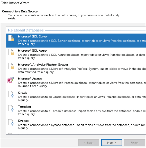
FIGURE 35.13 Activate the Table Import Wizard and select Microsoft SQL Server.
The Table Import Wizard will now ask for all the information it needs to connect to your chosen data source. This includes things such as server address, login credentials, and any other database name. The wizard will show you different fields based on the type of data source you select. The more common fields you'll see when connecting to an external data source are as follows:
- Friendly Connection Name The Friendly Connection Name field allows you to specify your own name for the external source. You typically enter a name that is descriptive and easy to read.
Server Name This is the name of the server that contains the database to which you are trying to connect. You will get this from your IT department when they give you access.
Log on to the Server These are your login credentials. Depending on how your IT department gives you access, you will select either Use Windows Authentication or Use SQL Server Authentication. The Use Windows Authentication option essentially means that the server will recognize you by your Windows login. The Use SQL Server Authentication option means that the IT department created a distinct username and password for you. If you select Use SQL Server Authentication, you will need to provide a username and password. Note that you will need at least
READprivileges for the target database to pull the needed data. - Save my Password You can select the check box next to Save my Password if you want your username and password to be stored in the workbook. This allows your connections to remain refreshable when being used by other people. There are obviously security issues with this option because anyone can view the connection properties and see your username and password. You should use this option only if your IT department set you up with an application account (that is, an account created specifically to be used by multiple people).
Database Name Every SQL Server can contain multiple databases. Enter the name of the database to which you are connecting. You will get this from your IT department when they give you access.
Once you enter all the pertinent information, click the Next button to get to the subsequent screen, as shown in Figure 35.14. Here you have the choice of selecting from a list of tables and views or writing your own custom query using SQL syntax. The latter involves writing your own SQL scripts. In most cases, you will choose the option to select from a list of tables.

FIGURE 35.14 Choose to select from a list of tables and views.
The Table Import Wizard reads the database and shows you a list of all available tables and views (see Figure 35.15). The tables will have an icon that looks like a grid, while views will have an icon that looks like a box on top of another box.

FIGURE 35.15 The Table Import Wizard will display a list of tables and views.
The idea is to place a check next to the tables and views that you want to import. The Friendly Name column allows you to enter a new name that will be used to reference the table in Power Pivot.
It's important to remember that importing a table imports all of the columns and records for that table. This can have an impact on the size and performance of your Power Pivot data model. You will often find that you need only a handful of the columns from the tables you import. In these cases, you can use the Preview & Filter button.
Click the table name to highlight it in blue (as shown in Figure 35.15) and then click the Preview & Filter button. The Table Import Wizard will activate the preview screen illustrated in Figure 35.16. In this screen, you will see all the columns available in the table, with a sampling of rows.

FIGURE 35.16 The Preview & Filter screen allows you to exclude columns and filter for only data you
Each column header has a check box next to it, indicating that the column will be imported with the table. Removing the check mark tells Power Pivot not to include that column in the data model.
You also have the option of filtering out certain records. Clicking the drop-down arrow illustrated in Figure 35.16 activates a filter menu that allows you to specify criteria to filter out unwanted records. This works just like the standard filtering in Excel.
Once you're done selecting your data and applying any needed filters, you can click the Finish button on the Table Import Wizard to start the import process. The import log shown in Figure 35.17 displays the progress of the import and summarizes the import actions taken after completion.

FIGURE 35.17 The last screen of the Table Import Wizard shows you the progress of your import actions.
The final step in loading data from SQL Server is to review and create any needed relationships. Activate the Power Pivot window and click the Diagram View button on the Home tab. Power Pivot will display the diagram screen where you can view and edit relationships as needed (see “Creating relationships between your Power Pivot tables” earlier in this chapter).
Loading data from other relational database systems
Whether your data lives in Microsoft Access, Oracle, dBase, or MySQL, you can load data from virtually any relational database system. As long as you have the appropriate database drivers installed, you have a way to connect Power Pivot to your data.
Activate the Power Pivot window, and click the From Other Sources button on the Home tab. This will activate the same Table Import Wizard as shown previously in Figure 35.13.
Select the appropriate relational database system from the plethora of options. If you need to import data from Oracle, select Oracle. If you need to import data from Sybase, select Sybase.
Connecting to any of these relational systems takes you through roughly the same steps you saw when importing SQL Server data earlier in this chapter. You may see some alternate dialog boxes, however, based on the needs of the database system you select.
Understandably, Microsoft cannot possibly create a named connection option for every database system out there. So, you may not find your database system listed. In this case, simply select the option called Others (OLEDB/ODBC). Selecting this option opens the Table Import Wizard starting with a screen asking you to enter the connection string for your database system.
Loading data from flat files
The term flat file refers to a file that contains some form of tabular data without any sort of structural hierarchy or relationship between records. The most common types of flat files are Excel files and text files. A ton of important data is maintained in flat files. In this section, you'll discover how to import these flat file data sources into the Power Pivot data model.
Loading data from external Excel files
Earlier in this chapter, you created linked tables by loading Power Pivot with the data contained within the same workbook. Linked tables have a distinct advantage over other types of imported data in that they immediately respond to changes in the source data within the workbook. If you change the data in one of the tables in the workbook, the linked table within the Power Pivot data model automatically changes. The real-time interactivity you get with linked tables is really nice to have.
The drawback to linked tables is that the source data must be kept in the same workbook as the Power Pivot data model. This isn't always possible. You'll encounter plenty of scenarios where you'll need to incorporate Excel data into your analysis but that data lives in another workbook. In these cases, you can use Power Pivot's Table Import Wizard to connect to external Excel files.
Activate the Power Pivot window and click the From Other Sources button on the Home tab. This will activate the Table Import Wizard dialog box. Scroll down and select the Excel File option in Figure 35.18 and then click the Next button.

FIGURE 35.18 Activate the Table Import Wizard and select Excel File.
The Table Import Wizard will now ask for all the information it needs to connect to your target workbook. In this screen, you'll need to provide the following:
- Friendly Connection Name The Friendly Connection Name field allows you to specify your own name for the external source. You typically enter a name that is descriptive and easy to read.
Excel File Path Enter the full path of your target Excel workbook. You can use the Browse button to search for and select the workbook from which you want to pull this information.
Use First Row as Column Headers In most cases, your Excel data will have column headers. Be sure to select the check box next to Use First Row as Column Headers to make sure that your column headers are recognized as headers when imported.
Once you enter all the pertinent information, click the Next button to get to the next screen, as shown in Figure 35.19. Here you'll see a list of all the worksheets in the chosen Excel workbook. Place a check mark next to the worksheets you want to import. The Friendly Name column allows you to enter a new name that will be used to reference the table in Power Pivot.

FIGURE 35.19 Select the worksheets you want to import.
As discussed earlier in this chapter, you can use the Preview & Filter button to filter out unwanted columns and records if needed. Otherwise, continue with the Table Import Wizard to complete the import process.
As always, be sure to review and create relationships to any other tables you've loaded into the Power Pivot data model.
Loading data from text files
Text files are another type of flat file used to distribute data. These files are commonly outputs from legacy systems and websites. Excel has always been able to import text files. With Power Pivot, you can go further and integrate them with other data sources.
Activate the Power Pivot window, and click the From Other Sources button on the Home tab. This will activate the same Table Import Wizard dialog box illustrated in Figure 35.18. Select the Text File option and then click the Next button.
The Table Import Wizard will ask for all the information it needs to connect to the target text file. In this screen, you'll need to provide the following:
- Friendly Connection Name The Friendly Connection Name field allows you to specify your own name for the external source. You typically enter a name that is descriptive and easy to read.
File Path Enter the full path of your target text file. You can use the Browse button to search for and select the file from which you want to pull this information.
Column Separator Select the character used to separate the columns in the text file. Before you can do this, you'll need to know how the columns in your text file are delimited. For instance, a comma-delimited file will have commas separating the columns. A tab-delimited file will have tabs separating the columns. The drop-down list in the Table Import Wizard includes choices for the more common delimiters: Tab, Comma, Semicolon, Space, Colon, and Vertical Bar.
Use First Row as Column Headers If your text file contains header rows, be sure to select the check box next to Use First Row as Column Headers. This ensures that the column headers are recognized as headers when imported.
You'll get an immediate preview of the data in the text file. As with other data sources we've covered here, you can filter out any unwanted columns simply by removing the check mark next to the column names. You can also use the drop-down arrows next to each column to apply any record filters.
Clicking the Finish button will immediately start the import process. Upon completion, the data from your text file will be part of the Power Pivot data model. As always, be sure to review and create relationships to any other tables that you've loaded into Power Pivot.
Loading data from the clipboard
Power Pivot includes an interesting option for loading data straight from the clipboard, that is, pasting data you've copied from some other place. This option is meant to be used as a one-off technique to get useful information into the Power Pivot data model quickly.
As you consider this option, keep in mind that there is no real data source. It's just you manually copying and pasting. There is no way to refresh the data, and there is no way to trace back where you actually copied the data from.
Imagine that you received a Word document showing a list of branches in a table. You'd like to include this static list of branches in your Power Pivot data model, as shown in Figure 35.20.

FIGURE 35.20 You can copy data straight out of Microsoft Word.
You can copy the table and then go to the Power Pivot window and click the Paste command on the Home tab. This activates the Paste Preview dialog box illustrated in Figure 35.21, where you can review what exactly will be pasted.

FIGURE 35.21 The Paste Preview dialog box gives you a chance to see what you're pasting.
There aren't that many options here. You can specify the name that will be used to reference the table in Power Pivot, and you can specify whether the first row is a header.
Clicking the OK button will import the pasted data into Power Pivot without a lot of fanfare. At this point, you can adjust the data formatting and create the needed relationships.
Refreshing and managing external data connections
When you load data from an external data source into Power Pivot, you essentially create a static snapshot of that data source at the time of creation. Power Pivot uses that static snapshot in its internal data model.
As time goes by, the external data source may change and grow with newly added records. However, Power Pivot is still using its snapshot, so it can't incorporate any of the changes in your data source until you take another snapshot.
The action of updating the Power Pivot data model by taking another snapshot of your data source is called refreshing your data. You can refresh manually, or you can set up an automatic refresh.
Manually refreshing your Power Pivot data
On the Home tab of the Power Pivot window, you will see the Refresh command. Clicking the drop-down arrow below it will display two options: Refresh and Refresh All.
Use the Refresh option to refresh the Power Pivot table that's currently active. That is, if you are on the Customers tab in Power Pivot, clicking Refresh will reach out to the external data source and request an update for just the Customers table. This works nicely when you need to refresh strategically only certain data sources.
Use the Refresh All option to refresh all the tables in the Power Pivot data model.
Setting up automatic refreshing
You can configure your data sources to pull the latest data and refresh Power Pivot automatically. Go to the Data tab in the Excel Ribbon, and select the Queries & Connections command. This will activate the Queries & Connections task pane illustrated in Figure 35.22.

FIGURE 35.22 The Queries & Connections task pane
Click Connections at the top of the task pane and then double-click the connection with which you want to work.
With the Connection Properties dialog box open (see Figure 35.23), select the Usage tab. Here you'll find the following options:

FIGURE 35.23 The Connection Properties dialog box lets you configure the chosen data connection to refresh automatically.
- Refresh Every X Minutes Placing a check mark next to this option tells Excel to refresh the chosen data connection automatically after a specified number of minutes. This will refresh all tables associated with that connection.
Refresh data when opening the file Placing a check mark next to this option tells Excel to refresh the chosen data connection automatically upon opening the workbook. This will refresh all tables associated with that connection as soon as the workbook is opened.
Refresh this connection on Refresh All Earlier in this section, you discovered that you can refresh all the connections that feed Power Pivot by using the Refresh All command found on the Power Pivot Home tab. If the data connection in question imports millions of lines of data from an external data source, you may not want to slow down your machine each time you trigger a Refresh All. You can remove the check mark next to the Refresh This Connection on Refresh All option. This essentially tells the connection to ignore the Refresh All command.
Editing your data connection
There may be instances where you need to edit your source data connection after you've already created it. Unlike refreshing, where you simply take another snapshot of the same data source, editing the source data connection allows you to go back and reconfigure the connection. Here are a few reasons that you'll need to edit a data connection:
In the Power Pivot window, go to the Home tab and click the Existing Connections button. The Existing Connections dialog box shown in Figure 35.24 will open. Your Power Pivot connections will be under the Power Pivot Data Connections subheading. Choose the data connection that needs editing.

FIGURE 35.24 Use the Existing Connections dialog box to reconfigure your Power Pivot source data connections.
Once your target data connection is selected, look to the Edit and Open buttons. The button you click depends on what you need to change.
- The Edit button Lets you reconfigure the server address, file path, and authentication settings.
The Open button Lets you import a new table from the existing connection. This is handy when you inadvertently missed a table during the initial loading of data.