
CHAPTER 38
Introducing Power Query
In information management, ETL refers to the three separate functions typically required to integrate disparate data sources: extraction, transformation, and loading. The extraction function refers to the reading of data from a specified source and extracting a desired subset of data. The transformation function refers to the cleaning, shaping, and aggregating of data to convert it to the desired structure. The loading function refers to the actual importing or writing of the resulting data to a target location.
Excel analysts have been manually performing ETL processes for years—although they rarely call it ETL. Every day, millions of Excel users manually pull data from some source location, manipulate that data, and integrate it into their reporting. This amounts to lots of manual effort.
Power Query enhances the ETL experience by offering an intuitive mechanism to extract data from a wide variety of sources, perform complex transformations on that data, and then load the data into a workbook or the internal data model.
In this chapter, you'll explore the basics of Power Query and get a glimpse of how it helps you save time and automate the steps needed to ensure that clean data is imported into your reporting models.
Understanding Power Query Basics
To start this basic look at Power Query, let's walk through a simple example. Imagine that you need to import Microsoft Corporation stock prices for the past 30 days using Yahoo Finance. For this scenario, you need to perform a web query to pull the data needed from Yahoo Finance.
To start your query, follow these steps:
- In Excel, select the Get Data command in the Get & Transform Data group on the Data tab and then select From Other Sources ⇨ From Web (see Figure 38.1).

FIGURE 38.1 Starting a Power Query web query
- In the dialog box that appears (see Figure 38.2), enter the URL for the data that you need, in this case,
http://finance.yahoo.com/q/hp?s=MSFT.
FIGURE 38.2 Enter the target URL containing the data you need.
After a bit of gyrating, the Navigator pane shown in Figure 38.3 appears. Here, you select the data source you want extracted. You can also click each table to see a preview of the data.

FIGURE 38.3 Select the correct data source and then click the Edit button.
- In this case, the table labeled Table 2 holds the historical stock data you need, so click Table 2 and then click the Edit button.
When you click the Edit button, Power Query activates a new Power Query Editor window, which contains its own Ribbon and a preview pane that shows a preview of the data (see Figure 38.4). Here, you can apply certain actions to shape, clean, and transform the data before importing.

FIGURE 38.4 The Power Query Editor window allows you to shape, clean, and transform data.
The idea is to work with each column shown in the Power Query Editor, applying the necessary actions that will give you the data and structure you need. You'll dive deeper into column actions later in this chapter. For now, you need to continue toward the goal of getting the last 30 days of stock prices for Microsoft Corporation.
- Right-click the Date field to see the available column actions, as shown in Figure 38.5. Select Change Type and then Date to ensure that the Date field is formatted as a proper date.

FIGURE 38.5 Right-click the Date column and choose to change the data type to a date format.
- Remove all the columns that you do not need by right-clicking each one and clicking Remove. (Besides the Date field, the only other columns that you need are the High, Low, and Close fields.) Alternatively, you can hold down the Ctrl key on your keyboard, select the columns you want to keep, right-click any of the selected columns, and then choose Remove Other Columns (see Figure 38.6).

FIGURE 38.6 Select the columns you want to keep and then select Remove Other Columns to get rid of the other columns.
- Ensure that the High, Low, and Close fields are formatted as proper numbers. To do this, hold down the Ctrl key on your keyboard, select the three columns, right-click one of the column headings, and then select Change Type ⇨ Decimal Number. After you do this, you may notice that some of the rows show the word Error. These are rows that contained text values that could not be converted.
- Remove the Error rows by selecting Remove Errors from the Column Actions list (next to the High field), as shown in Figure 38.7.
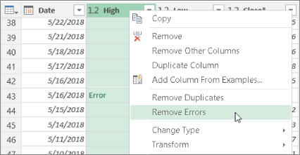
FIGURE 38.7 You can click the Table Actions icon to select actions (such as Remove Errors) that you want applied to the entire data table.
- Once all the errors are removed, add a Week Of field that displays the week to which each date in the table belongs. To do this, right-click the Date field and select the Duplicate Column option. A new column (named Date -Copy) is added to the preview.
- Right-click the newly added column, select the Rename option, and then rename the column
Week Of. - Right-click the Week Of column you just created and select the Transform ⇨ Week ⇨ Start of Week, as shown in Figure 38.8. Excel transforms the date to display the start of the week for a given date.

FIGURE 38.8 The Power Query Editor can be used to apply transformation actions such as displaying the start of the week for a given date.
- When you've finished configuring your Power Query feed, save and output the results. To do this, click the Close & Load drop-down found on the Home tab of the Power Query Ribbon to reveal the two options shown in Figure 38.9.

FIGURE 38.9 The Load To dialog box gives you more control over how the results of queries are used.
The Close & Load option saves your query and outputs the results to a new worksheet in your workbook as an Excel table. The Close & Load To option activates the Import Data dialog box, where you can choose to output the results to a specific worksheet or to the internal data model.
The Import Data dialog box also enables you to save the query as a query connection only, which means you will be able to use the query in various in-memory processes without actually needing to output the results anywhere. Select the New Worksheet option button to output your results as a table on a new worksheet in the active workbook.
At this point, you will have a table similar to the one shown in Figure 38.10, which can be used to produce the PivotTable you need.
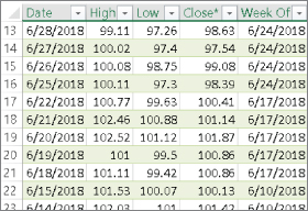
FIGURE 38.10 Your final query pulled from the Internet: transformed, put into an Excel table, and ready to use in a PivotTable
Take a moment to appreciate what Power Query allowed you to do just now. With a few clicks, you searched the Internet, found some base data, shaped the data to keep only the columns you needed, and even manipulated that data to add an extra Week Of dimension to the base data. This is what Power Query is about: enabling you easily to extract, filter, and reshape data without the need for any programmatic coding skills.
Understanding query steps
Power Query uses its own formula language, known as the M language, to codify your queries. As with macro recording, each action you take when working with Power Query results in a line of code being written into a query step. Query steps are embedded M code, which allows your actions to be repeated each time you refresh your Power Query data.
You can see the query steps for your queries by activating the Query Settings pane in the Power Query Editor window (see Figure 38.11). Simply click the Query Settings command on the View tab of the Ribbon. You can also place a check in the Formula Bar option to enhance your analysis of each step with a formula bar that displays the syntax for the given step.

FIGURE 38.11 Query steps can be viewed and managed in the Applied Steps section of the Query Settings pane.
Each query step represents an action that you took to get to a data table. You can click any step to see the underlying M code in the Power Query formula bar. For example, clicking the step called Removed Errors reveals the code for that step in the Formula bar.
You can right-click any step to see a menu of options for managing your query steps. Figure 38.12 illustrates the following options:

FIGURE 38.12 Right-click any query step to edit, rename, delete, or move the step.
- Edit Settings Edit the arguments or parameters that define the selected step.
RenameGive the selected step a meaningful name.
Delete Remove the selected step. Be aware that removing a step can cause errors if subsequent steps depend on the deleted step.
Delete Until End Remove the selected step and all following steps.
Move Up Move the selected step up in the order of steps.
Move Down Move the selected step down in the order of steps.
Extract Previous Extract all steps prior to this one into a new query.
Viewing the Advanced Query Editor
Power Query gives you the option of viewing and editing a query's embedded M code directly. While in the QPower Query Editor window, click the View tab of the Ribbon and select Advanced Editor. The Advanced Editor dialog box is little more than a space for you to edit the existing M code or type your own M code. Advanced users can use the M language to extend the capabilities of Power Query by directly coding their own steps in the Advanced Editor. We'll touch on the M language in Chapter 39, “Transforming Data with Power Query.”
Refreshing Power Query data
It's important to note that Power Query data is not in any way connected to the source data used to extract it. A Power Query data table is merely a snapshot. In other words, as the source data changes, Power Query will not automatically keep up with the changes; you intentionally need to refresh your query.
If you chose to load your Power Query results to an Excel table in the existing workbook, you can manually refresh by right-clicking the table and selecting the Refresh option.
If you chose to load your Power Query data to the internal data model, you need to click Data ⇨ Queries & Connections and then right-click the target query and select the Refresh option.
To get a bit more automated with the refreshing of your queries, you can configure your data sources to refresh your Power Query data automatically. To do so, follow these steps:
- Go to the Data tab in the Excel Ribbon, and click the Queries & Connections command. The Queries & Connections task pane appears.
- Right-click the Power Query data connection that you want to refresh and then select the Properties option.
- With the Properties dialog box open, select the Usage tab.
- Set the options to refresh the chosen data connection:
Refresh Every X Minutes Placing a check next to this option tells Excel to refresh the chosen data automatically every specified number of minutes. Excel will refresh all tables associated with that connection.
Refresh Data When Opening the File Placing a check next to this option tells Excel to refresh the chosen data connection automatically upon opening the workbook. Excel will refresh all tables associated with that connection as soon as the workbook is opened.
These refresh options are useful when you want to ensure that your customers are working with the latest data. Of course, setting these options does not preclude the ability to refresh the data manually.
Managing existing queries
As you add various queries to a workbook, you will need a way to manage them. Excel accommodates this need by offering the Queries & Connections pane, which enables you to edit, duplicate, refresh, and generally manage all of the existing queries in the workbook. Activate the Queries & Connections pane by selecting the Queries & Connections command on the Data tab of the Excel Ribbon.
You need to find the query on which you want to work and then right-click it to take any one of the following actions (see Figure 38.13):

FIGURE 38.13 Right-click any query in the Queries & Connections pane to see the available management options.
- Edit Open the Power Query Editor, where you can modify the query steps.
DeleteDelete the selected query.
Rename Rename the selected query.
Refresh Refresh the data in the selected query.
Load To Open the Load To dialog box, where you can redefine where the selected query's results are used.
Duplicate Create a copy of the query.
Reference Create a new query that references the output of the original query.
Merge Merge the selected query with another query in the workbook by matching specified columns.
Append Append the results of another query in the workbook to the selected query.
Send To Data Catalog Publish and share the selected query via a Power BI server that your IT department sets up and manages.
Export Connection File Save an Office Data Connection (
.odc) file with the connection credentials for the query's source data.Move To Group Move the selected query into a logical group that you create for better organization.
Move Up Move the selected query up in the Queries & Connections pane.
Move Down Move the selected query down in the Queries & Connections pane.
Show the Peek Show a preview of the query results for the selected query.
Properties Rename the query and add a friendly description.
The Queries & Connections pane is especially useful when your workbook contains several queries. Think of it as a kind of table of contents that allows you to easily find and interact with the queries in your workbook.
Understanding column-level actions
Right-clicking a column in the Power Query Editor activates a shortcut menu that shows a full list of the actions you can take. You can also apply certain actions to multiple columns at one time by selecting two or more columns before right-clicking. Figure 38.14 shows the available column-level actions, and Table 38.1 explains them, as well as a few other actions that are available only in the Power Query Editor Ribbon.

FIGURE 38.14 Right-click any column to see the column-level actions that you can use to transform the data.
TABLE 38.1 Column-Level Actions
| Action | Purpose | Available with Multiple Columns? |
| Remove | Remove the selected column from the Power Query data. | Yes |
| Remove Other Columns | Remove all nonselected columns from the Power Query data. | Yes |
| Duplicate Column | Create a duplicate of the selected column as a new column placed at the far right of the table. The name given to the new column is Copy of X, where X is the name of the original column. | No |
| Add Column From Examples | Create a custom column that combines data from other columns based on a few examples that you provide. Like the Flash Fill feature in Excel, Power Query's smart detection logic infers transformation logic based on your examples and then applies that logic to fill the new column. | Yes |
| Remove Duplicates | Remove all rows from the selected column where the values duplicate earlier values. The row with the first occurrence of a value is not removed. | Yes |
| Remove Errors | Remove rows containing errors in the selected column. | Yes |
| Change Type | Change the data type of the selected column. | Yes |
| Transform | Change the way values in the column are rendered. You can choose from the following options: Lowercase, Uppercase, Capitalize Each Word, Trim, Clean, Length, JSON, and XML. If the values in the column are date/time values, the options are as follows: Date, Time, Day, Month, Year, or Day of Week. If the values in the column are number values, the options are as follows: Round, Absolute Value, Factorial, Base-10 Logarithm, Natural Logarithm, Power, or Square Root. | Yes |
| Replace Values | Replace one value in the selected column with another specified value. | Yes |
| Replace Errors | Replace unsightly error values with your own friendlier text. | Yes |
| Group By | Aggregate data by row values. For example, you can group by state and either count the number of cities in each state or sum the population of each state. | Yes |
| Fill | Fill empty cells in the column with the value of the first nonempty cell. You have the option of filling up or filling down. | Yes |
| Unpivot Columns | Transpose the selected columns from column-oriented to row-oriented or vice versa. | Yes |
| Unpivot Other Columns | Transpose the unselected columns from column-oriented to row-oriented or vice versa. | Yes |
| Unpivot Only Selected Columns | Transpose the selected columns from column-oriented to row-oriented or vice versa. This option also retains a columns list in the current step so that the same set of columns is unpivoted on future refresh operations. | Yes |
| Rename | Rename the selected column to a name you specify. | No |
| Move | Move the selected column to a different location in the table. You have these choices for moving the column: Left, Right, To Beginning, and To End. | Yes |
| Drill Down | Navigate to the contents of the column. This is used with tables that contain metadata representing embedded information. | No |
| Add as New Query | Create a new query with the contents of the column. This is done by referencing the original query in the new one. The name of the new query is the same as the column header of the selected column. | No |
| Split Column (Ribbon only) | Split the value of a single column into two or more columns, based on a number of characters or a given delimiter, such as a comma, semicolon, or tab. | No |
| Merge Column (Ribbon only) | Merge the values of two or more columns into a single column that contains a specified delimiter, such as a comma, semicolon, or tab. | Yes |
Understanding table actions
While you're in the Power Query Editor, Power Query allows you to apply certain actions to an entire data table. You can see the available table-level actions by clicking the Table Actions icon, as shown in Figure 38.15.

FIGURE 38.15 Click the Table Actions icon in the upper-left corner of the Power Query Editor Preview pane to see the table-level actions you can use to transform the data.
Table 38.2 lists the table-level actions and describes the primary purpose of each one.
TABLE 38.2 Table-Level Actions
| Action | Purpose |
| Copy Entire Table | Copy the data within the current query to the Clipboard. |
| Use First Row as Headers | Replace each table header name with the value in the first row of each column. |
| Add Custom Column | Insert a new column after the last column of the table. The values in the new column are determined by the value or formula you define. |
| Add Column From Examples | Create a custom column that combines data from other columns based on a few examples that you provide. Like the Flash Fill feature in Excel, Power Query's smart detection logic infers transformation logic based on your examples and then applies that logic to fill the new column. |
| Invoke Custom Function | Insert a new column after the last column of the table and then run a user-defined function for each row in the column. |
| Add Conditional Column | Insert a new column after the last column of the table and then fill it with a conditional if-then-else statement that you define. |
| Add Index Column | Insert a new column containing a sequential list of numbers starting from 1, 0, or another specified value you define. |
| Choose Columns | Choose the columns you want to keep in the query results. |
| Keep Top Rows | Remove all but the top N number of rows. You specify the number threshold. |
| Keep Bottom Rows | Remove all but the bottom N number of rows. You specify the number threshold. |
| Keep Range of Rows | Remove all rows except the ones that fall within a range you specify. |
| Keep Duplicates | Remove all rows where the values in the selected columns are unique, enabling you to focus on the duplicate rows. |
| Keep Errors | Remove all rows that do not contain an error. This allows for the quick filtering of error values encountered during transformation. |
| Remove Top Rows | Remove the top N rows from the table. |
| Remove Bottom Rows | Remove the bottom N rows from the table. |
| Remove Alternate Rows | Remove alternate rows from the table, starting at the first row to remove and specifying the number of rows to remove and the number of rows to keep. |
| Remove Duplicates | Remove all rows where the values in the selected columns duplicate earlier values. The row with the first occurrence of a value set is not removed. |
| Remove Errors | Remove rows containing errors in the currently selected columns. |
| Merge Queries | Create a new query that merges the current table with another query in the workbook by matching specified columns. |
| Append Queries | Create a new query that appends the results of another query in the workbook to the current table. |
Getting Data from External Sources
Microsoft has invested a great deal of time and resources in ensuring that Power Query has the ability to connect to a wide array of data sources. Whether you need to pull data from an external website, a text file, a database system, Facebook, or a web service, Power Query can accommodate most, if not all, data sources.
You can see all the available connection types by clicking the Get Data drop-down on the Data tab in the Excel Ribbon. As Figure 38.16 illustrates, Power Query offers the ability to pull from a wide array of data sources.

FIGURE 38.16 Power Query has the ability to connect to a wide array of text, database, and Internet data sources.
- From File Pulls data from a specified Excel file, text file, CSV file, XML file, JSON file, or folder.
From Azure Pulls data from Microsoft's Azure Cloud service.
From Database Pulls data from databases like Microsoft Access, SQL Server, or SQL Server Analysis Services.
From Online Services Pulls data from cloud application services such as Facebook, Salesforce, and Microsoft Dynamics online.
From Other Sources Pulls data from a wide array of Internet, cloud, and other ODBC data sources. Here, you will also find the Blank Query option. Selecting Blank Query will activate the Power Query Editor in the Advanced Editor view. This is handy when you want to copy and paste M code directly into the Power Query Editor.
In the rest of this chapter, you will explore the various connection types that can be leveraged to import external data.
Importing data from files
Organizational data is often kept in files such as text files, CSV files, and even other Excel workbooks. It's not uncommon to use these kinds of files as data sources for data analysis. Power Query offers several connection types that enable the importing of data from external files.
Getting data from Excel workbooks
You can import data from other Excel workbooks by going to the Excel Ribbon and selecting Data ⇨ Get Data ⇨ From File ⇨ From Workbook.
Note that you can import any kind of Excel file, including macro-enabled workbooks and template workbooks. Power Query will not bring in charts, PivotTables, shapes, VBA code, or any other objects that may exist within a workbook. It simply imports the data found in the used cell ranges of the workbook.
Once you've selected your file, the Navigator pane will activate, showing you all of the data sources available in the workbook. The idea here is to select the data source you want and then either load or edit the data using the buttons at the bottom of the Navigator pane. The Load button allows you to skip any editing and import your targeted data as is. Use the Edit button if you want to transform or shape the data before completing the import.
In terms of Excel workbooks, a data source is either a worksheet or a defined named range. The icons next to each data source let you distinguish those sources that are worksheets and those that are named ranges. In Figure 38.17, the source called MyNamedRange is a defined named range, while the source called National Parks is a worksheet.

FIGURE 38.17 Select the data sources with which you want to work and then click the Load button.
You can import multiple sources at once by clicking the Select multiple items check box and then placing a check next to each worksheet and named range that you want to import.
Getting data from CSV and text files
Text files are commonly used to store and distribute data because of their inherent ability to hold many thousands of bytes of data without having an inflated file size. Text files can do this by forgoing all the fancy formatting, leaving only the text.
Comma-separated value (CSV) files are text files that contain commas to delimit (separate) values into columns of data.
To import a text or CSV file, go to the Excel Ribbon and select Data ⇨ Get Data ⇨ From File ⇨ From Text/CSV. Excel will activate the Import Data dialog box where you can browse for and select a text or CSV file.
Power Query will open the Power Query Editor to show you the contents of the text or CSV file that you just imported. The idea here is to apply any changes you want to make to the data and then click the Close & Load command on the Home tab to complete the import.
Power Query is good at recognizing the correct delimiters in CSV files and typically does a good job of importing the data correctly.
For instance, row 5 in the sample CSV file illustrated in Figure 38.18 contains the value Johnson, Kimberly. Power Query contains the intelligence to know that the comma in that value is not an actual delimiter. So, all of the columns are separated correctly.

FIGURE 38.18 CSV files are brought into the Power Query Editor where you can apply your edits and then click the Close & Load command to complete the import.
Importing data from database systems
In larger organizations, the task of data management is not performed by Excel; rather, it is primarily performed by database systems such as Microsoft Access and SQL Server. Databases like these not only store millions of rows of data but also ensure data integrity, prevent redundancy, and allow for the rapid search and retrieval of data through queries and views.
Power Query offers options to connect to a wide array of database types. Microsoft has been keen to add connection types for as many commonly used databases as it can.
Importing data from relational and OLAP databases
Click Data ⇨ Get Data ⇨ From Database, and you will see the list of databases to which you can connect. Power Query offers connection types for many of the popular database systems in use today: SQL Server, Microsoft Access, Oracle, MySQL, and so on.
Importing data from Azure databases
If your organization has a Microsoft Azure cloud database or a subscription to Microsoft Azure Marketplace, there is an entire set of connection types designed to import data from Azure. You can get to these connection types by clicking Data ⇨ Get Data ⇨ From Azure.
Importing data using ODBC connections to nonstandard databases
Some of you may be using a unique nonstandard database system that isn't popular enough to be specifically included as an option under the Get Data command. Not to worry. As long as an ODBC connection string can be used to connect to your database system, Power Query can connect to it.
Click Data ⇨ Get Data ⇨ From Other Sources to see a list of other connection types. Click the From ODBC option to start a connection to your unique database via an ODBC connection string.
Getting Data from Other Data Systems
In addition to ODBC, Figure 38.19 illustrates other kinds of data systems that can be leveraged by Power Query.

FIGURE 38.19 Other systems Power Query can utilize as data sources
To get to the list shown in Figure 38.19, select Data ⇨ Get Data ⇨ From Other Data Sources. Some of these data systems (SharePoint, Active Directory, and Microsoft Exchange) are popular ones that are used in many organizations to store data, track sales opportunities, and manage email. Other systems like OData Feed and Hadoop are less-common services used to work with large volumes of data. These are often mentioned in conversations about “Big Data.” Of course, the From Web option (demonstrated earlier in this chapter) is an integral connection type for any analyst who leverages data from the Internet.
Clicking any of these connections will activate a set of dialog boxes customized for the selected connection. These dialog boxes ask for the basic parameters that Power Query needs to connect to the specified data source; they are parameters such as file path, URL, server name, credentials, and so forth.
Each connection type requires its own unique set of parameters, so each of their dialog boxes will be different. Luckily, Power Query rarely needs more than a handful of parameters to connect to any one data source, so the dialog boxes are relatively intuitive and hassle-free.
Managing Data Source Settings
Each time you connect to any web-based data source or data source that requires some level of credentials, Power Query caches (stores) the settings for that data source.
For instance, let's say you connected to a SQL Server database, entered all of your credentials, and imported the data you needed. At the moment of successful connection, Power Query caches information about that connection in a file located on your local PC. This includes connection string, username, password, privacy settings, and so on.
The purpose of all this caching is so that you don't have to re-enter credentials each time you need to refresh your queries. That's nifty, but what happens when your credentials are changed? Well, the short answer is those queries will fail until the data source settings are updated.
Editing data source settings
You can edit data source settings by activating the Data Source Settings dialog box. To do so, click Data ⇨ Get Data ⇨ Data Source Settings.
The Data Source Settings dialog box, shown in Figure 38.20, contains a list of all credentials-based data sources previously used in queries. Select the data source you need to change and then click the Edit Permissions button.

FIGURE 38.20 Edit a data source by selecting it and clicking the Edit button.
Another dialog box will pop up, this one specific to the data source you selected (see Figure 38.21). This dialog box enables you to edit credentials as well as other data privacy settings.

FIGURE 38.21 The credentials edit screen for your selected data source
Click the Edit button to make changes to the credentials for the data source. The credentials edit screen will differ based on the data source with which you are working, but again, the input dialog boxes are relatively intuitive and easy to update.