Chapter 13
Ten Ways to Improve Power Pivot Performance
In This Chapter
![]() Improving Power Pivot performance
Improving Power Pivot performance
![]() Best practices for avoiding lag
Best practices for avoiding lag
![]() Managing slicer performance
Managing slicer performance
![]() Using views versus tables
Using views versus tables
When you publish Power Pivot reports to the web, you intend to give your audience the best experience possible. A large part of that experience is ensuring that performance is good.
The word performance (as it relates to applications and reporting) is typically synonymous with speed — or how quickly an application performs certain actions such as opening within the browser, running queries, or filtering.
Because Power Pivot inherently paves the way for large amounts of data with fairly liberal restrictions, it isn’t uncommon to produce reporting solutions that work but are unbearably slow. And nothing will turn your intended audience away from your slick new reports faster than painfully sluggish performance.
This chapter offers ten actions you can take to optimize the performance of your Power Pivot reports.
Limit the Number of Rows and Columns in Your Data Model Tables
One huge influence on Power Pivot performance is the number of columns you bring, or import, into the data model. Every column you import is one more dimension that Power Pivot has to process when loading a workbook. Don’t import extra columns “just in case” — if you’re not certain you will use certain columns, just don’t bring them in. These columns are easy enough to add later if you find that you need them.
 More rows mean more data to load, more data to filter, and more data to calculate. Avoid selecting an entire table if you don’t have to. Use a query or a view at the source database to filter for only the rows you need to import. After all, why import 400,000 rows of data when you can use a simple WHERE clause and import only 100,000?
Use Views Instead of Tables
Speaking of views, for best practice, use views whenever possible.
Though tables are more transparent than views — allowing you to see all the raw, unfiltered data — they come supplied with all available columns and rows, whether you need them or not. To keep your Power Pivot data model to a manageable size, you’re often forced to take the extra step of explicitly filtering out the columns you don’t need.
Views can not only provide cleaner, more user-friendly data but also help streamline your Power Pivot data model by limiting the amount of data you import.
Avoid Multi-Level Relationships
Both the number of relationships and the number of relationship layers have an impact on the performance of your Power Pivot reports. When building your model, follow best practice and have a single fact table containing primarily quantitative numerical data (facts) and dimension tables that relate to the facts directly. In the database world, this configuration is a star schema, as shown in Figure 13-1.

Figure 13-1: A star schema is the most efficient data model, with a single fact table and dimensions relating directly to it.
 Avoid building models where dimension tables relate to other dimension tables. Figure 13-2 illustrates this configuration, also known as a snowflake schema. This configuration forces Power Pivot to perform relationship lookups across several dimension levels, which can be particularly inefficient, depending on the volume of data in the model.
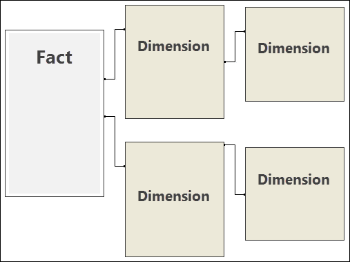
Figure 13-2: Snowflake schemas are less efficient, causing Power Pivot to perform chain lookups.
Let the Back-End Database Servers Do the Crunching
Most Excel analysts who are new to Power Pivot tend to pull raw data directly from the tables on their external database servers. After the raw data is in Power Pivot, they build calculated columns and measures to transform and aggregate the data as needed. For example, users commonly pull revenue and cost data and then create a calculated column in Power Pivot to compute profit.
So why make Power Pivot do this calculation when the back-end server could have handled it? The reality is that back-end database systems such as SQL Server have the ability to shape, aggregate, clean, and transform data much more efficiently than Power Pivot. Why not utilize their powerful capabilities to massage and shape data before importing it into Power Pivot?
Rather than pull raw table data, consider leveraging queries, views, and stored procedures to perform as much of the data aggregation and crunching work as possible. This leveraging reduces the amount of processing that Power Pivot will have to do and naturally improves performance.
Beware of Columns with Non-Distinct Values
Columns that have a high number of unique values are particularly hard on Power Pivot performance. Columns such as Transaction ID, Order ID, and Invoice Number are often unnecessary in high-level Power Pivot reports and dashboards. So unless they are needed to establish relationships to other tables, leave them out of your model.
Limit the Number of Slicers in a Report
The slicer is one of the best new business intelligence (BI) features of Excel in recent years. Using slicers, you can provide your audience with an intuitive interface that allows for interactive filtering of your Excel reports and dashboards.
One of the more useful benefits of the slicer is that it responds to other slicers, providing a cascading filter effect. For example, Figure 13-3 illustrates not only that clicking on Midwest in the Region slicer filters the pivot table but that the Market slicer also responds, by highlighting the markets that belong to the Midwest region. Microsoft calls this behavior cross-filtering.
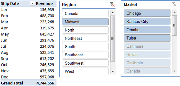
Figure 13-3: Slicers work together to show relevant data items based on a selection.
As useful as the slicer is, it is, unfortunately, extremely bad for Power Pivot performance. Every time a slicer is changed, Power Pivot must recalculate all values and measures in the pivot table. To do that, Power Pivot must evaluate every tile in the selected slicer and process the appropriate calculations based on the selection.
Take this process a step further and imagine adding a second slicer: Because slicers cross-filter, each time you click one slicer, the other one changes also, so it’s almost as though you clicked both of them. Power Pivot must now respond to both slicers, evaluating every tile in both slicers for each calculated measure in the pivot. Adding a second slicer effectively doubles the processing time. Add a third slicer, and you triple the processing time.
In short, a slicer is generally bad for Power Pivot performance. However, as mentioned at the beginning of this section, the functionality that the slicer brings to Excel BI solutions is too good to give up completely.
You can help to mitigate performance issues by limiting the number of slicers in your Power Pivot reports. Remove slicers one at a time, testing the performance of the Power Pivot report after each removal. You‘ll find that removing a single slicer is often enough to correct performance issues.
Remove slicers that have low click rates. Some slicers hold filter values that, frankly, may never be utilized by your audience. For example, if a slicer allows your audience to filter by the current year or by last year, and the last year view is not often called up, consider removing the slicer or using the Pivot Table Filter drop-down list instead.
Create Slicers Only on Dimension Fields
Slicers tied to columns that contain lots of unique values will often cause a larger performance hit than columns containing only a handful of values. If a slicer contains a large number of tiles, consider using a Pivot Table Filter drop-down list instead.
On a similar note, be sure to right-size column data types. A column with few distinct values is lighter than a column with a high number of distinct values. If you’re storing the results of a calculation from a source database, reduce the number of digits (after the decimal) to be imported. This reduces the size of the dictionary and, possibly, the number of distinct values.
Disable the Cross-Filter Behavior for Certain Slicers
Disabling the cross-filter behavior of a slicer essentially prevents that slicer from changing selections when other slicers are clicked. This prevents the need for Power Pivot to evaluate the titles in the disabled slicer, thus reducing processing cycles. To disable the cross-filter behavior of a slicer, select Slicer Settings to open the Slicer Settings dialog box, shown in Figure 13-4. Then simply deselect the Visually Indicate Items with No Data option.
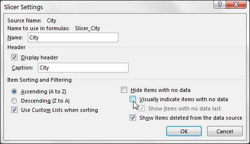
Figure 13-4: Deselecting the Visually Indicate Items option with No Data disables the slicer’s cross-filter behavior.
Use Calculated Measures Instead of Calculated Columns
Use calculated measures instead of calculated columns, if possible. Calculated columns are stored as imported columns. Because calculated columns inherently interact with other columns in the model, they calculate every time the pivot table updates, whether they are being used or not. Calculated measures, on the other hand, calculate only at query time.
Calculated columns resemble regular columns in that they both take up space in the model. In contrast, calculated measures are calculated on the fly and do not take space.
Upgrade to 64-Bit Excel
The suggestion in this section is somewhat obvious. If you continue to run into performance issues with your Power Pivot reports, you can always buy a better PC — in this case, by upgrading to a 64-bit PC with 64-bit Excel installed.
Power Pivot loads the entire data model into RAM whenever you work with it. The more RAM your computer has, the fewer performance issues you see. The 64-bit version of Excel can access more of your PC’s RAM, ensuring that it has the system resources needed to crunch through bigger data models. In fact, Microsoft recommends 64-bit Excel for anyone working with models made up of millions of rows.
But before you hurriedly start installing 64-bit Excel, you need to answer these questions:
- Do you already have 64-bit Excel installed? In Excel 2016 and 2013, choose File ⇒ Account ⇒ About Excel. A dialog box opens, specifying either 32-bit or 64-bit at the top. In Excel 2010, choose File ⇒ Help instead. The text About Excel pops up on the right side of the screen along with the version number and the 32-bit or 64-bit designation.
- Are your data models large enough? Unless you’re working with large data models, the move to 64-bit may not produce a noticeable difference in your work. How large is large? A Power Pivot workbook with a file size upward of 40 megabytes is considered large. If your workbook is 50 or more megabytes, you would definitely benefit from an upgrade.
- Do you have a 64-bit operating system installed on your PC? The 64-bit version of Excel will not install on a 32-bit operating system. You can find out whether you’re running a 64-bit operating system by searching for the text My PC 64-bit or 32-bit at your favorite search engine. You’ll see loads of sites that can walk you through the steps to determine your version.
- Will your other add-ins stop working? If you’re using other add-ins, be aware that some of them may not be compatible with 64-bit Excel. You wouldn’t want to install 64-bit Excel just to find that your trusted add-ins no longer work. Contact your add-in providers to ensure that they are 64-bit compatible. By the way, this advice includes add-ins for all Office products — not just Excel. When you upgrade Excel to 64-bit, you also have to upgrade the entire Office suite.