
Chapter 4
Using External Data with Power Pivot
In This Chapter
![]() Importing from relational databases
Importing from relational databases
![]() Importing from flat files
Importing from flat files
![]() Importing data from other data sources
Importing data from other data sources
![]() Refreshing and managing external data connections
Refreshing and managing external data connections
In Chapter 2, I start an exploration of Power Pivot by showing you how to load the data already contained within the workbook you’re working on. But as you discover in this chapter, you’re not limited to using only the data that already exists in your Excel workbook.
Power Pivot has the ability to reach outside the workbook and import data found in external data sources. Indeed, what makes Power Pivot powerful is its ability to consolidate data from disparate data sources and build relationships between them. You can theoretically create a Power Pivot data model that contains some data from a SQL Server table, some data from a Microsoft Access database, and even data from a one-off text file.
In this chapter, I help you continue your journey by taking a closer look at the mechanics of importing external data into your Power Pivot data models.
 This chapter has no associated sample file. But don’t worry: You can easily translate the information found here to your own data sources.
Loading Data from Relational Databases
One of the more common data sources used by Excel analysts is the relational database. It’s not difficult to find an analyst who frequently uses data from Microsoft Access, SQL Server, or Oracle databases. In this section, I walk you through the steps for loading data from external database systems.
Loading data from SQL Server
SQL Server databases are some of the most commonly used for the storing of enterprise-level data. Most SQL Server databases are managed and maintained by the IT department. To connect to a SQL Server database, you have to work with your IT department to obtain Read access to the database you’re trying to pull from.
After you have access to the database, open the Power Pivot window and click the From Other Sources command button on the Home tab. This opens the Table Import Wizard dialog box, shown in Figure 4-1. There, select the Microsoft SQL Server option and then click the Next button.

Figure 4-1: Open the Table Import Wizard and select Microsoft SQL Server.
The Table Import Wizard now asks for all the information it needs to connect to your database (see Figure 4-2). On this screen, you need to provide the information for the options described in this list:
- Friendly Connection Name: The Friendly Name field allows you to specify your own name for the external source. You typically enter a name that is descriptive and easy to read.
- Server Name: This is the name of the server that contains the database you’re trying to connect to. You get this from your IT department when you gain access. (Your server name will be different from the one shown in Figure 4-2.)
- Log On to the Server: These are your login credentials. Depending on how your IT department gives you access, you select either Windows Authentication or SQL Server Authentication. Windows Authentication essentially means that the server recognizes you by your windows login. SQL Server Authentication means that the IT department created a distinct username and password for you. If you’re using SQL Server Authentication, you need to provide a username and password.
- Save My Password: You can select the check box next to Save My Password if you want your username and password to be stored in the workbook. Your connections can then remain refreshable when being used by other people. This option obviously has security considerations, because anyone can view the connection properties and see your username and password. You should use this option only if your IT department has set you up with an application account (an account created specifically to be used by multiple people).
- Database Name: Every SQL Server can contain multiple databases. Enter the name of the database you’re connecting to. You can get it from your IT department whenever someone gives you access.
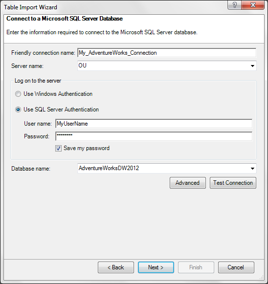
Figure 4-2: Provide the basic information needed to connect to the target database.
After you enter all the pertinent information, click the Next button to see the next screen, shown in Figure 4-3. You have the choice of selecting from a list of tables and views or writing your own custom query using SQL syntax. In most cases, you choose the option to select from a list of tables.

Figure 4-3: Choose to select from a list of tables and views.
The Table Import Wizard reads the database and shows you a list of all available tables and views (see Figure 4-4). Tables have an icon that looks like a grid, and views have an icon that looks like a box on top of another box.

Figure 4-4: The Table Import Wizard offers up a list of tables and views.
The idea is to place a check mark next to the tables and views you want to import. In Figure 4-4, note the check mark next to the FactInternetSales table. The Friendly Name column allows you to enter a new name that will be used to reference the table in Power Pivot.
 In Figure 4-4, you see the Select Related Tables button. After you select one or more tables, you can click this button to tell Power Pivot to scan for, and automatically select, any other tables that have a relationship with the table(s) you’ve already selected. This feature is handy to have when sourcing large databases with dozens of tables.
Importing a table imports all columns and records for that table. This can have an impact on the size and performance of your Power Pivot data model. You will often find that you need only a handful of the columns from the tables you import. In these cases, you can use the Preview & Filter button.
Click the table name to highlight it in blue (refer to Figure 4-4), and then click the Preview & Filter button. The Table Import Wizard opens the Preview Selected Table screen, shown in Figure 4-5. You can see all columns available in the table, with a sampling of rows.

Figure 4-5: The Preview & Filter screen allows you to filter out columns you don’t need.
Each column header has a check box next to it, indicating that the column will be imported with the table. Removing the check mark tells Power Pivot to not include that column in the data model.
You also have the option to filter out certain records. Figure 4-6 demonstrates that clicking on the drop-down arrow for any of the columns opens a Filter menu that allows you to specify criterion to filter out unwanted records. This works just like the standard filtering in Excel. You can select and deselect the data items in the filtered list, or, if there are too many choices, you can apply a broader criteria by clicking Date Filters above the list. (If you’re filtering a textual column, it’s Text Filters.)

Figure 4-6: Use the drop-down arrows in each column to filter out unneeded records.
After you finish selecting your data and applying any needed filters, you can click the Finish button on the Table Import Wizard to start the import process. The import log, shown in Figure 4-7, shows the progress of the import and summarizes the import actions taken after completion.

Figure 4-7: The last screen of the Table Import Wizard shows you the progress of your import actions.
The final step in loading data from SQL Server is to review and create any needed relationships. Open the Power Pivot window and click the Diagram View command button on the Home tab. Power Pivot opens the diagram screen (see Figure 4-8), where you can view and edit relationships as needed.

Figure 4-8: Be sure to review and create any needed relationships.
Don’t panic if you feel like you’ve botched the column-and-record filtering on your imported Power Pivot table. Simply select the worrisome table in the Power Pivot window and open the Edit Table Properties dialog box (choose Design ⇒ Table Properties). Note that this dialog box is basically the same Preview & Filter screen you encounter in the Import Table Wizard (refer to Figure 4-5). From here, you can select columns you originally filtered out, edit record filters, clear filters, or even use a different table/view.
Chapter 2 tells you more about relationships.
Loading data from Microsoft Access databases
Because Microsoft Access has traditionally been made available with the Microsoft Office suite of applications, Access databases have long been used by organizations to store and manage mission-critical departmental data. Walk into any organization, and you will likely find several Access databases that contain useful data.
Unlike SQL Server databases, Microsoft Access databases are typically found on local desktops and directories. This means you can typically import data from Access without the help of your IT department.
Open the Power Pivot window and click the From Other Sources command button on the Home tab. This opens the Table Import Wizard dialog box, shown in Figure 4-9. Select the Microsoft Access option, and then click the Next button.

Figure 4-9: Open the Table Import Wizard and select Microsoft Access.
The Table Import Wizard asks for all the information it needs to connect to your database (see Figure 4-10).

Figure 4-10: Provide the basic information needed to connect to the target database.
On this screen, you need to provide the information for these options:
- Friendly Connection Name: The Friendly Name field allows you to specify your own name for the external source. You typically enter a name that is descriptive and easy to read.
- Database Name: Enter the full path of your target Access database. You can use the Browse button to search for and select the database you want to pull from.
- Log On to the Database: Most Access databases aren’t password protected. But if you’re connecting one that does require a username and password, enter your login credentials.
Save My Password: You can select the check box next to Save My Password if you want your username and password to be stored in the workbook. Then your connections can remain “refreshable” when being used by other people. Keep in mind that anyone can view the connection properties and see your username and password.
 Because Access databases are essentially desktop files (.mdb or .accdb), they’re susceptible to being moved, renamed, or deleted. Be aware that the connections in your workbook are hard coded, so if you do move, rename, or delete your Access database, you can no longer connect it.
At this point, you can click the Next button to continue with the Table Import Wizard. From here on out, the process is virtually identical to importing SQL Server data, covered in the last section (starting at Figure 4-3).
Loading data from other relational database systems
Whether your data lives in Oracle, Dbase, or MySQL, you can load data from virtually any relational database system. As long as you have the appropriate database drivers installed, you have a way to connect Power Pivot to your data.
Open the Power Pivot window and click the From Other Sources command button on the Home tab. This opens the Table Import Wizard dialog box, shown in Figure 4-11. The idea is to select the appropriate relational database system. If you need to import data from Oracle, select Oracle. If you need to import data from Sybase, select Sybase.

Figure 4-11: Open the Table Import Wizard and select your target relational database system.
Connecting to any of these relational systems takes you through roughly the same steps as importing SQL Server data, earlier in this chapter. You may see some alternative dialog boxes based on the needs of the database system you select.
Understandably, Microsoft cannot possibly create a named connection option for every database system out there. So you may not find your database system listed. In this case, simply select the Others option (OLEDB/ODBC). Selecting this option opens the Table Import Wizard, starting with a screen asking you to enter or paste the connection string for your database system (see Figure 4-12).

Figure 4-12: Enter the connection string for your database system.
You may be able to get this connection string from your IT department. If you’re having trouble finding the correct syntax for your connection string, you can use the Build button to create the string via a set of dialog boxes. Pressing the Build button opens the Data Link Properties dialog box, shown in Figure 4-13.

Figure 4-13: Use the Data Link Properties dialog box to configure a custom connection string to your relational database system.
Start with the Provider tab, selecting the appropriate driver for your database system. The list you see on your computer will be different from the list shown in Figure 4-13. Your list will reflect the drivers you have installed on your own machine.
After selecting a driver, move through each tab on the Data Link Properties dialog box and enter the necessary information. When it’s complete, click OK to return to the Table Import Wizard, where you see the connection string input box populated with the connection string needed to connect to your database system (see Figure 4-14).

Figure 4-14: The Table Import Wizard displays the final syntax for your connection string.
Again, from here on out, the process is virtually identical to importing SQL Server data, as covered earlier in this chapter (starting at Figure 4-3).
To connect to any database system, you must have that system’s drivers installed on your PC. Because SQL Server and Access are Microsoft products, their drivers are virtually guaranteed to be installed on any PC with Windows installed. The drivers for other database systems, however, need to be explicitly installed — typically, by the IT department either at the time the machine is loaded with corporate software or upon demand. If you don’t see the needed drivers for your database system, contact your IT department.
Loading Data from Flat Files
The term flat file refers to a file that contains some form of tabular data without any sort of structural hierarchy or relationship between records. The most common types of flat files are Excel files and text files. Whether anyone likes to admit it or not, a ton of important data is maintained in flat files. In this section, I tell you how to import these flat file data sources into the Power Pivot data model.
Loading data from external Excel files
In Chapter 2, I show you how to create linked tables by loading Power Pivot with the data contained within the same workbook. Linked tables have a distinct advantage over other types of imported data in that they immediately respond to changes in the source data within the workbook. If you change the data in one of the tables in the workbook, the linked table within the Power Pivot data model automatically changes. The real-time interactivity you get with linked tables is especially helpful if you’re making frequent changes to your data.
The drawback to linked tables is that the source data must be stored in the same workbook as the Power Pivot data model. This isn’t always possible. You’ll encounter plenty of scenarios where you need to incorporate Excel data into your analysis, but that data lives in another workbook. In these cases, you can use Power Pivot’s Table Import Wizard to connect to external Excel files.
Open the Power Pivot window and click the From Other Sources command button on the Home tab. This opens the Table Import Wizard dialog box, shown in Figure 4-15. Select the Excel File option and then click the Next button.

Figure 4-15: Open the Table Import Wizard and select Excel File.
The Table Import Wizard asks for all the information it needs to connect to your target workbook (see Figure 4-16).

Figure 4-16: Provide the basic information needed to connect to the target workbook.
On this screen, you need to provide the following information:
- Friendly Connection Name: In the Friendly Connection Name field, you specify your own name for the external source. You typically enter a name that is descriptive and easy to read.
- Excel File Path: Enter the full path of your target Excel workbook. You can use the Browse button to search for and select the workbook you want to pull from.
- Use First Row as Column Headers: In most cases, your Excel data will have column headers. Select the check box next to Use First Row As Column Headers to ensure that your column headers are recognized as headers when imported.
After you enter all the pertinent information, click the Next button to see the next screen, shown in Figure 4-17. You see a list of all worksheets in the chosen Excel workbook. In this case, you have only one worksheet. Place a check mark next to the worksheets you want to import. The Friendly Name column allows you to enter a new name that will be used to reference the table in Power Pivot.

Figure 4-17: Select the worksheets to import.
When reading from external Excel files, Power Pivot cannot identify individual table objects. As a result, you can select only entire worksheets in the Table Import Wizard (shown in Figure 4-17). Keeping this in mind, make sure to import worksheets that contain a single range of data.
As discussed earlier in this chapter, in the section “Loading Data from Relational Databases,” you can use the Preview & Filter button to filter out unwanted columns and records, if needed. Otherwise, continue with the Table Import Wizard to complete the import process.
As always, be sure to review and create relationships to any other tables you’ve loaded into the Power Pivot data model.
Loading external Excel data doesn’t give you the same interactivity you get with linked tables. As with importing database tables, the data you bring from an external Excel file is simply a snapshot. You need to refresh the data connection to see any new data that may have been added to the external Excel file (see “Refreshing and Managing External Data Connections,” later in this chapter).
Loading data from text files
The text file is another type of flat file used to distribute data. This type of file is commonly output from legacy systems and websites. Excel has always been able to consume text files. With Power Pivot, you can go further and integrate them with other data sources.
Open the Power Pivot window and click the From Other Sources command button on the Home tab. This opens the Table Import Wizard dialog box shown in Figure 4-18. Select the Text File option and then click the Next button.

Figure 4-18: Open the Table Import Wizard and select Excel File.
The Table Import Wizard asks for all the information it needs to connect to the target text file (see Figure 4-19).

Figure 4-19: Provide the basic information needed to connect to the target text file.
On this screen, you provide the following information:
- Friendly Connection Name: The Friendly Connection Name field allows you to specify your own name for the external source. You typically enter a name that is descriptive and easy to read.
- File Path: Enter the full path of your target text file. You can use the Browse button to search for and select the file you want to pull from.
- Column Separator: Select the character used to separate the columns in the text file. Before you can do this, you need to know how the columns in your text file are delimited. For instance, a comma-delimited file will have commas separating its columns. A tab-delimited file will have tabs separating the columns. The drop-down list in the Table Import Wizard includes choices for the more common delimiters: Tab, Comma, Semicolon, Space, Colon, and Vertical bar.
- Use First Row as Column Headers: If your text file contains header rows, be sure to select the check box next to Use First Row as a Column Headers. This ensures that the column headers are recognized as headers when imported.
Notice that you see an immediate preview of the data in the text file. Here, you can filter out any unwanted columns by simply removing the check mark next to the column names. You can also use the drop-down arrows next to each column to apply any record filters.
Clicking the Finish button immediately starts the import process. Upon completion, the data from your text file will be part of the Power Pivot data model. As always, be sure to review and create relationships to any other tables you’ve loaded into Power Pivot.
Anyone who’s worked with text files in Excel knows that they’re notorious for importing numbers that look like numbers, but are really coded as text. In standard Excel, you use Text to Columns to fix these kinds of issues. Well, this can be a problem in Power Pivot, too.
When importing text files, take the extra step of verifying that all columns have been imported with the correct data formatting. You can use the formatting tools found on the Power Pivot window’s Home tab to format any column in the data model.
Loading data from the Clipboard
Power Pivot includes an interesting option for loading data straight from the Clipboard — that is to say, pasting data you’ve copied from some other place. This option is meant to be used as a one-off technique to quickly get useful information into the Power Pivot data model.
As you consider this option, keep in mind that there is no real data source. It’s just you manually copying and pasting. You have no way to refresh the data, and you have no way to trace back to where you copied the data from.
Imagine that you’ve received the Word document shown in Figure 4-20. You like the nifty table of holidays within the document, and you believe it would be useful in your Power Pivot data model.

Figure 4-20: You can copy data straight out of Microsoft Word.
You can copy the table and then go to the Power Pivot window and click the Paste command on the Home tab. This opens the Past Preview dialog box, shown in Figure 4-21, where you can review what exactly will be pasted. You won’t see many options here. You can specify the name that will be used to reference the table in Power Pivot, and you can specify whether the first row is a header.

Figure 4-21: The Paste Preview dialog box gives you a chance to see what you’re pasting.
Clicking the OK button imports the pasted data into Power Pivot without a lot of fanfare. At this point, you can adjust the data formatting and create the needed relationships.
Loading Data from Other Data Sources
At this point, I’ve covered the data sources that are most important to a majority of Excel analysts. Still, there are a few more data sources that Power Pivot is able to connect to and load data from. I touch on some of these data sources later in this book, though others remain out of scope.
Although these data sources are not likely to be used by your average analyst, it’s worth dedicating a few lines to each one, if only to know that they exist and are available if ever you should need them:
- Microsoft SQL Azure: SQL Azure is a cloud-based relational database service that some companies use as an inexpensive way to gain the benefits of SQL Server without taking on the full cost of hardware, software, and IT staff. Power Pivot can load data from SQL Azure in much the same way as the other relational databases I talk about in this chapter.
- Microsoft SQL Parallel Data Warehouse: SQL Parallel Data Warehouse (SQL PDW) is an appliance that partitions very large data tables into separate servers and manages query processing between them. SQL PDW is used to provide scalability and performance for big data analytics. From a Power Pivot perspective, it’s no different than connecting to any other relational database.
- Microsoft Analysis Services: Analysis Services is Microsoft’s OLAP (Online Analytical Processing) product. The data in Analysis Services is traditionally stored in a multidimensional cube.
- Report: The curiously named Report data source refers to SQL Server Reporting Services reports. In a very basic sense, Reporting Services is a business intelligence tool used to create stylized PDF-style reports from SQL Server data. In the context of Power Pivot, a Reporting Services Report can be used as a data-feed service, providing a refreshable connection to the underlying SQL Server data.
- From Windows Azure Marketplace: Windows Azure Marketplace is an OData (Open Data Protocol) service that provides both free and paid data sources. Register for a free Azure Marketplace account and you get instant access to governmental data, industrial market data, consumer data, and much more. You can enhance your Power Pivot analyses by loading the data from the Azure marketplace using this connection type.
- Suggested Related Data: This data source reviews the content of the Power Pivot data model and, based on its findings, suggests Azure Marketplace data that you may be interested in.
- Other Feeds: The Other Feeds data source allows you to import data from OData web services into Power Pivot. OData connections are facilitated by XML Atom files. Point the OData connection to the URL of the .atomsvcs file and you essentially have a connection to the published web service.
Refreshing and Managing External Data Connections
When you load data from an external data source into Power Pivot, you essentially create a static snapshot of that data source at the time of creation. Power Pivot uses that static snapshot in its Internal Data Model.
As time goes by, the external data source may change and grow with newly added records. However, Power Pivot is still using its snapshot, so it can’t incorporate any of the changes in your data source until you take another snapshot.
The action of updating the Power Pivot data model by taking another snapshot of your data source is called refreshing the data. You can refresh manually, or you can set up an automatic refresh.
Manually refreshing Power Pivot data
On the home tab of the Power Pivot window, you see the Refresh command. Click the drop-down arrow below it to see two options shown in Figure 4-22: Refresh and Refresh All.

Figure 4-22: Power Pivot allows you to refresh one table or all tables.
Use the Refresh option to refresh the Power Pivot table that’s active. That is to say, if you’re on the Dim_Products tab in Power Pivot, clicking Refresh reaches out to the external SQL Server and requests an update for only the Dim_Products table. This works nicely when you need to strategically refresh only certain data sources.
Use the Refresh All option to refresh all tables in the Power Pivot data model.
Setting up automatic refreshing
You can configure your data sources to automatically pull the latest data and refresh Power Pivot.
Go to the Data tab on the Excel Ribbon, and select the Connections command. The Workbook Connections dialog box, shown in Figure 4-23, opens. Select the data connection you want to work with and then click the Properties button.

Figure 4-23: Select a connection and click the Properties button.
With the Properties dialog box open, select the Usage tab. Here, you’ll find an option to refresh the chosen data connection every X minutes and an option to refresh the data connection when the Excel work is opened (see Figure 4-24):
- Refresh Every X Minutes: Placing a check next to this option tells Excel to automatically refresh the chosen data connection a specified number of minutes. This refreshes all tables associated with that connection.
- Refresh Data When Opening the File: Placing a check mark next to this option tells Excel to automatically refresh the chosen data connection after opening of the workbook. This refreshes all tables associated with that connection as soon as the workbook is opened.

Figure 4-24: The Properties dialog box lets you configure the chosen data connection to refresh automatically.
Preventing Refresh All
Earlier in this section, you see that you can refresh all connections that feed Power Pivot, by using the Refresh All command (refer to Figure 4-22). Well, there are actually two more places where you can click Refresh All in Excel: on the Data tab in the Excel Ribbon and on the Analyze tab you see when working in a pivot table.
In Excel 2010, these two buttons refreshed only standard pivot tables and workbook data connections, and the Power Pivot refresh buttons affected only Power Pivot. They now all trigger the same operation. So clicking any Refresh All button anywhere in Excel essentially completely reloads Power Pivot, refreshes all pivot tables, and updates all workbook data connections. If your Power Pivot data model imports millions of lines of data from an external data source, you may well want to avoid using the Refresh All feature.
Luckily, you have a way to prevent certain data connections from refreshing when Refresh All is selected. Go to the Data tab on the Excel Ribbon and select the Connections command. This opens the Workbook Connections dialog box, where you select the data connection you want to configure, and then click the Properties button.
When the Properties dialog box has opened, select the Usage tab and then remove the check mark next to the Refresh This Connection on Refresh All (as shown in Figure 4-25).

Figure 4-25: The Properties dialog box lets you configure the chosen data connection to ignore the Refresh All command.
Editing the data connection
In certain instances, you may need to edit the source data connection after you’ve already created it. Unlike refreshing, where you simply take another snapshot of the same data source, editing the source data connection allows you to go back and reconfigure the connection itself. Here are a few reasons you may need to edit the data connection:
- The location or server or data source file has changed.
- The name of the server or data source file has changed.
- You need to edit your login credentials or authentication mode.
- You need to add tables you left out during initial import.
In the Power Pivot window, go to the Home tab and click the Existing Connections command button. The Existing Connections dialog box, shown in Figure 4-26, opens. Your Power Pivot connections are under the Power Pivot Data Connections subheading. Choose the data connection that needs editing.

Figure 4-26: Use the Existing Connections dialog box to reconfigure your Power Pivot source data connections.
After your target data connection is selected, look to the Edit and Open buttons. The button you click depends on what you need to change:
- Edit button: Lets you reconfigure the server address, file path, and authentication settings.
- Open button: Lets you import a new table from the existing connection, which is handy when you’ve inadvertently missed a table during the initial loading of data.