
Chapter 2
Introducing Power Pivot
In This Chapter
![]() Getting to know the Internal Data Model
Getting to know the Internal Data Model
![]() Activating the Power Pivot add-in
Activating the Power Pivot add-in
![]() Linking to Excel data
Linking to Excel data
![]() Managing relationships
Managing relationships
Over the past decade or so, corporate managers, eager to turn impossible amounts of data into useful information, drove the business intelligence (BI) industry to innovate new ways of synthesizing data into meaningful insights. During this period, organizations spent lots of time and money implementing big enterprise reporting systems to help keep up with the hunger for data analytics and dashboards.
Recognizing the importance of the BI revolution and the place that Excel holds within it, Microsoft proceeded to make substantial investments in improving Excel’s BI capabilities. It specifically focused on Excel’s self-service BI capabilities and its ability to better manage and analyze information from the increasing number of available data sources.
The key product of that endeavor was essentially Power Pivot (introduced in Excel 2010 as an add-In). With Power Pivot came the ability to set up relationships between large, disparate data sources. For the first time, Excel analysts were able to add a relational view to their reporting without the use of problematic functions such as VLOOKUPS. The ability to merge data sources with hundreds of thousands of rows into one analytical engine within Excel was groundbreaking.
With the release of Excel 2016, Microsoft incorporated Power Pivot directly into Excel. The powerful capabilities of Power Pivot are available out of the box!
In this chapter, you get an overview of those capabilities by exploring the key features, benefits, and capabilities of Power Pivot.
Understanding the Power Pivot Internal Data Model
At its core, Power Pivot is essentially a SQL Server Analysis Services engine made available by way of an in-memory process that runs directly within Excel. Its technical name is the xVelocity analytics engine. However, in Excel, it’s referred to as the Internal Data Model.
Every Excel workbook contains an Internal Data Model, a single instance of the Power Pivot in-memory engine. The most effective way to interact with the Internal Data Model is to use the Power Pivot Ribbon interface, which becomes available when you activate the Power Pivot Add-In.
The Power Pivot Ribbon interface exposes the full set of functionality you don’t get with the standard Excel Data tab. Here are a few examples of functionality available with the Power Pivot interface:
- You can browse, edit, filter, and apply custom sorting to data.
- You can create custom calculated columns that apply to all rows in the data import.
- You can define a default number format to use when the field appears in a pivot table.
- You can easily configure relationships via the handy Graphical Diagram view.
- You can choose to prevent certain fields from appearing in the Pivot Table Field List.
As with everything else in Excel, the Internal Data Model does have limitations. Most Excel users will not likely hit these limitations, because Power Pivot’s compression algorithm is typically able to shrink imported data to about one-tenth its original size. For example, a 100MB text file would take up only approximately 10MB in the Internal Data Model.
Nevertheless, it’s important to understand the maximum and configurable limits for Power Pivot Data Models. Table 2-1 highlights them.
Table 2-1 Limitations of the Internal Data Model
Object |
Specification |
Data model size |
In 32-bit environments, Excel workbooks are subject to a 2GB limit. This includes the in-memory space shared by Excel, the Internal Data Model, and add-ins that run in the same process. In 64-bit environments, there are no hard limits on file size. Workbook size is limited only by available memory and system resources. |
Number of tables in the data model |
No hard limits exist on the count of tables. However, all tables in the data model cannot exceed 2,147,483,647 bytes. |
Number of rows in each table in the data model |
1,999,999,997 |
Number of columns and calculated columns in each table in the data model |
The number cannot exceed 2,147,483,647 bytes. |
Number of distinct values in a column |
1,999,999,997 |
Characters in a column name |
100 characters |
String length in each field |
It’s limited to 536,870,912 bytes (512MB), equivalent to 268,435,456 Unicode characters (256 mega-characters). |
Data model size |
In 32-bit environments, Excel workbooks are subject to a 2GB limit. This includes the in-memory space shared by Excel, the Internal Data Model, and add-ins that run in the same process. In 64-bit environments, no hard limits on file size exist. Workbook size is limited only by available memory and system resources. |
Number of tables in the data model |
No hard limits exist on the count of tables. However, all tables in the data model cannot exceed 2,147,483,647 bytes. |
Number of rows in each table in the data model |
1,999,999,997 |
Number of columns and calculated columns in each table in the data model |
The number cannot exceed 2,147,483,647 bytes. |
Number of distinct values in a column |
1,999,999,997 |
Characters in a column name |
100 characters |
String length in each field |
It’s limited to 536,870,912 bytes (512MB), equivalent to 268,435,456 Unicode characters (256 mega-characters). |
Data model size |
In 32-bit environments, Excel workbooks are subject to a 2GB limit. This includes the in-memory space shared by Excel, the Internal Data Model, and add-ins that run in the same process. |
Activating the Power Pivot Add-In
As mentioned earlier in this chapter, the Power Pivot Ribbon interface is available only when you activate the Power Pivot Add-In. The Power Pivot Add-In does not install with every edition of Office. For example, if you have Office Home Edition, you cannot see or activate the Power Pivot Add-In and therefore cannot have access to the Power Pivot Ribbon interface.
As of this writing, the Power Pivot Add-In is available to you only if you have one of these editions of Office or Excel:
- Office 2013 or 2016 Professional Plus: Available only through volume licensing
- Office 365 Pro Plus: Available with an ongoing subscription to Office365.com
- Excel 2013 or Excel 2016 Stand-alone Edition: Available for purchase via any retailer
If you have any of these editions, you can activate the Power Pivot add-in by following these steps:
Open Excel and look for the Power Pivot tab on the Ribbon.
If you see the tab, the Power Pivot add-in is already activated. You can skip the remaining steps.
- Go to the Excel Ribbon and choose File ⇒ Options.
- Choose the Add-Ins option on the left, and then look at the bottom of the dialog box for the Manage drop-down list. Select COM Add-Ins from that list, and then click Go.
- Look for Microsoft Office Power Pivot for Excel in the list of available COM add-ins, and select the check box next to this option. Click OK.
- If the Power Pivot tab does not appear in the Ribbon, close Excel and restart.
After installing the add-in, you should see the Power Pivot tab on the Excel Ribbon, as shown in Figure 2-1.

Figure 2-1: When the add-in has been activated, you see a new Power Pivot tab on the Ribbon.
Linking Excel Tables to Power Pivot
The first step in using Power Pivot is to fill it with data. You can either import data from external data sources or link to Excel tables in your current workbook. I cover importing data from external data sources in Chapter 3. For now, let me start this walkthrough by showing you how to link three Excel tables to Power Pivot.
 You can find the sample file for this chapter on this book’s companion website at
 www.dummies.com/go/excelpowerpivotpowerqueryfd in the workbook named Chapter 2 Samples.xlsx.
In this scenario, you have three data sets in three different worksheets: Customers, InvoiceHeader, and InvoiceDetails (see Figure 2-2).

Figure 2-2: You want to use Power Pivot to analyze the data in the Customers, InvoiceHeader, and InvoiceDetails worksheets.
The Customers data set contains basic information, such as CustomerID, Customer Name, and Address. The InvoiceHeader data set contains data that points specific invoices to specific customers. The InvoiceDetails data set contains the specifics of each invoice.
To analyze revenue by customer and month, it’s clear that you first need to somehow join these three tables together. In the past, you would have to go through a series of gyrations involving VLOOKUP or other clever formulas. But with Power Pivot, you can build these relationships in just a few clicks.
Preparing Excel tables
When linking Excel data to Power Pivot, best practice is to first convert the Excel data to explicitly named tables. Although not technically necessary, giving tables friendly names helps track and manage your data in the Power Pivot data model. If you don't convert your data to tables first, Excel does it for you and gives your tables useless names like Table1, Table2, and so on.
Follow these steps to convert each data set into an Excel table:
- Go to the Customers tab and click anywhere inside the data range.
Press Ctrl+T on the keyboard.
This step opens the Create Table dialog box, shown in Figure 2-3.
In the Create Table dialog box, ensure that the range for the table is correct and that the My Table Has Headers check box is selected. Click the OK button.
You should now see the Table Tools Design tab on the Ribbon.
Click the Table Tools Design tab, and use the Table Name input to give your table a friendly name, as shown in Figure 2-4.
This step ensures that you can recognize the table when adding it to the Internal Data Model.
- Repeat Steps 1 through 4 for the Invoice Header and Invoice Details data sets.

Figure 2-3: Convert the data range into an Excel table.

Figure 2-4: Give your newly created Excel table a friendly name.
Adding Excel Tables to the data model
After you convert your data to Excel tables, you’re ready to add them to the Power Pivot data model. Follow these steps to add the newly created Excel tables to the data model using the Power Pivot tab:
- Place the cursor anywhere inside the Customers Excel table.
- Go to the Power Pivot tab on the Ribbon and click the Add to Data Model command.
Power Pivot creates a copy of the table and opens the Power Pivot window, shown in Figure 2-5.
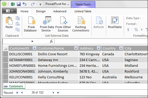
Figure 2-5: The Power Pivot window shows all the data that exists in your data model.
Although the Power Pivot window looks like Excel, it’s a separate program altogether. Notice that the grid for the Customers table has no row or column references. Also notice that you cannot edit the data within the table. This data is simply a snapshot of the Excel table you imported.
Additionally, if you look at the Windows taskbar at the bottom of the screen, you can see that Power Pivot has a separate window from Excel. You can switch between Excel and the Power Pivot window by clicking each respective program on the taskbar.
Repeat Steps 1 and 2 in the preceding list for your other Excel tables: Invoice Header, Invoice Details. After you’ve imported all your Excel tables into the data model, the Power Pivot window will show each dataset on its own tab, as shown in Figure 2-6.
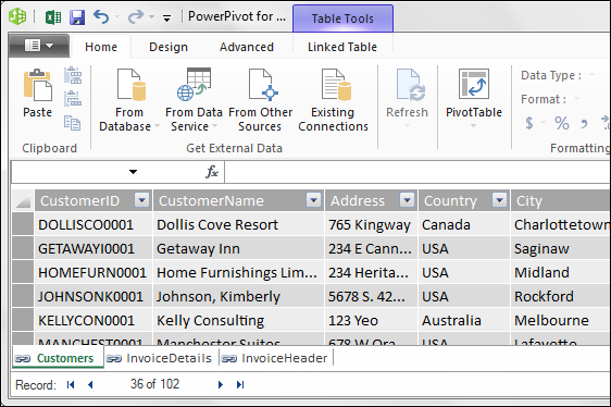
Figure 2-6: Each table you add to the data model is placed on its own tab in Power Pivot.
 The tabs in the Power Pivot window shown in Figure 2-6 have a Hyperlink icon next to the tab names, indicating that the data contained in the tab is a linked Excel table. Even though the data is a snapshot of the data at the time you added it, the data automatically updates whenever you edit the source table in Excel.
Creating relationships between Power Pivot tables
At this point, Power Pivot knows that you have three tables in the data model but has no idea how the tables relate to one another. You connect these tables by defining relationships between the Customers, Invoice Details, and Invoice Header tables. You can do so directly within the Power Pivot window.
 If you’ve inadvertently closed the Power Pivot window, you can easily reopen it by clicking the Manage command button on the Power Pivot Ribbon tab.
Follow these steps to create relationships between your tables:
Activate the Power Pivot window and click the Diagram View command button on the Home tab.
The Power Pivot screen you see shows a visual representation of all tables in the data model, as shown in Figure 2-7.
You can move the tables in Diagram view by simply clicking and dragging them.The idea is to identify the primary index keys in each table and connect them. In this scenario, the Customers table and the Invoice Header table can be connected using the CustomerID field. The Invoice Header and Invoice Details tables can be connected using the InvoiceNumber field.
- Click and drag a line from the CustomerID field in the Customers table to the CustomerID field in the Invoice Header table, as demonstrated in Figure 2-8.
- Click and drag a line from the InvoiceNumber field in the Invoice Header table to the InvoiceNumber field in the Invoice Details table.

Figure 2-7: Diagram view allows you to see all tables in the data model.

Figure 2-8: To create a relationship, you simply click and drag a line between the fields in your tables.
At this point, your diagram will look similar to Figure 2-9. Notice that Power Pivot shows a line between the tables you just connected. In database terms, these are referred to as joins.

Figure 2-9: When you create relationships, the Power Pivot diagram shows join lines between tables.
The joins in Power Pivot are always one-to-many joins. This means that when a table is joined to another, one of the tables has unique records with unique index numbers, while the other can have many records where index numbers are duplicated.
A common example, illustrated in Figure 2-9, is the relationship between the Customers table and the Invoice Header table. In the Customers table, you have a unique list of customers, each with its own, unique identifier. No CustomerID in that table is duplicated. The Invoice header table has many rows for each CustomerID; each customer can have many invoices.
Notice that the join lines have arrows pointing from a table to another table. The arrow in these join lines always points to the table that has the duplicated unique index.
To close the diagram and return to seeing the data tables, click the Data View command in the Power Pivot window.
Managing existing relationships
If you need to edit or delete a relationship between two tables in your data model, you can do so by following these steps:
- Open the Power Pivot window, select the Design tab, and then select the Manage Relationships command.
- In the Manage Relationships dialog box, shown in Figure 2-10, click the relationship you want to work with and click Edit or Delete.
- If you clicked Edit, the Edit Relationship dialog box appears, as shown in Figure 2-11. Use the drop-down and list box controls on this form to select the appropriate table and field names to redefine the relationship.

Figure 2-10: Use the Manage Relationships dialog box to edit or delete existing relationships.

Figure 2-11: Use the Edit Relationship dialog box to adjust the tables and field names that define the selected relationship.
In Figure 2-11, you see a graphic of an arrow between the list boxes. The graphic has an asterisk next to the list box on the left, and a number 1 next to the list box on the right. The number 1 basically indicates that the model will use the table listed on the right as the source for a unique primary key.
Every relationship must have a field that you designate as the primary key. Primary key fields are necessary in the data model to prevent aggregation errors and duplications. In that light, the Excel data model must impose some strict rules around the primary key.
You cannot have any duplicates or null values in a field being used as the primary key. So the Customers table (refer to Figure 2-11) must have all unique values in the CustomerID field, with no blanks or null values. This is the only way that Excel can ensure data integrity when joining multiple tables.
At least one of your tables must contain a field that serves as a primary key — that is, a field that contains only unique values and no blanks.
Using the Power Pivot data model in reporting
After you define the relationships in your Power Pivot data model, it’s essentially ready for action. In terms of Power Pivot, action means analysis with a pivot table. In fact, all Power Pivot data is presented through the framework of pivot tables.
In Chapter 3, you dive deep into the workings of pivot tables. For now, dip just a toe in and create a simple pivot table from your new Power Pivot data model:
- Activate the Power Pivot window, select the Home tab, and then click the Pivot Table command button.
- Specify whether you want the pivot table placed on a new worksheet or an existing sheet.
- Build out the needed analysis just as you would build out any other standard pivot table, using the Pivot Field List.
The pivot table shown in Figure 2-12 contains all tables in the Power Pivot data model. In this configuration, you essentially have a powerful cross-table analytical engine in the form of a familiar pivot table. Here, you can see that you’re calculating the average unit price by customer.

Figure 2-12: You now have a Power Pivot-driven pivot table that aggregates across multiple tables.
In the days before Power Pivot, this analysis would have been a bear to create. You would have had to build VLOOKUP formulas to get from Customer Number to Invoice Number, and then another set of VLOOKUP formulas to get from Invoice Numbers to Invoice Details. And after all that formula building, you still would have had to find a way to aggregate the data to the average unit price per customer.