C H A P T E R  3

Hybrid Columnar Compression

Hybrid Columnar Compression (HCC) is probably one of the least understood of the features that are unique to Exadata. The feature was originally rolled out in a beta version of 11gR2 and was enabled on both Exadata and non-Exadata platforms. The production release of 11gR2 restricted the feature to Exadata platforms only. Ostensibly this decision was made because the additional processing power available on the Exadata storage servers. Because the feature is restricted to Exadata, the recent documentation refers to it as Exadata Hybrid Columnar Compression (EHCC).

This chapter will first present basic information on both of Oracle’s older row-major format compression methods (BASIC and OLTP). We will then explore in detail the mechanics of Oracle’s new HCC feature—how it works, including how the data is actually stored on disk, where and when the compression and decompression occur, and when its use is appropriate. Finally we’ll provide some real world examples of HCC usage.

Oracle Storage Review

As you probably already know, Oracle stores data in a block structure. These blocks are typically 8K and from a simplistic point of view they consist of a block header, a row directory, row data and free space. The block header starts at the top of a block and works its way down, while the row data starts at the bottom and works its way up. The free space generally sits in the middle. Figure 3-1 shows a representation of a traditional Oracle block format.

Figure 3-1. The standard Oracle block format (row-major storage)

Rows are stored in no specific order, but columns are generally stored in the order in which they were defined in the table. For each row in a block there will be a row header, followed by the column data for each column. Figure 3.2 shows how the pieces of a row are stored in a standard Oracle block. Note that we called it a row piece, because occasionally a row’s data may be stored in more than one chunk. In this case, there will be a pointer to the next piece.

Figure 3-2. The standard Oracle row format (row-major storage)

Note that the row header may contain a pointer to another row piece. We’ll come back to this a little later, but for now, just be aware that there is a mechanism to point to another location. Also note that each column is preceded by a separate field indicating the length of the column. Nothing is actually stored in the Column Value field for nulls. The presence of a null column is indicated by a value of 0 in the column length field. Trailing nulls don’t even store the column length fields, as the presence of a new row header indicates that there are no more columns with values in the current row.

PCTFREE is a key value associated with blocks; it controls how space is used in a block. Its purpose is to reserve some free space in each block for updates. This is necessary to prevent row migration (moving rows to new blocks) that would be caused by lack of space in the row’s original block when a row increases in size. When rows are expected to be updated (with values that require more space), more space is generally reserved. When rows are not expected to increase in size because of updates, values as low as 0 may be specified for PCTFREE. With compressed blocks it is common to use very low values of PCTFREE, because the goal is to minimize space usage and the rows are generally not expected to be updated frequently (if ever). Figure 3-3 shows how free space is reserved based on the value of PCTFREE.

Figure 3-3. Block free space controlled by PCTFREE

Figure 3-3 shows a block that reserves 20 percent of its space for updates. A block with a PCTFREE setting of 0 percent would allow inserts to fill the block almost completely. When a record is updated, and the new data will not fit in the available free space of the block where the record is stored, the database will move the row to a new block. This process is called row migration. It does not completely remove the row from the original block but leaves a reference to the newly relocated row so that it can still be found by its original rowid (which basically consists of a file number, block number, and row number within the block). This ability of Oracle to relocate rows will become relevant when we discuss what happens if you update a row that has been compressed. Note that the more generic term for storing rows in more than one piece is row chaining. Row migration is a special case of row chaining in which the entire row is relocated. Figure 3-4 shows what a block with a migrated row might look like.

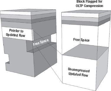
Figure 3-4. Row migration

This diagram represents a situation where the entire row has been relocated, leaving behind only a pointer to the new location.

Oracle Compression Mechanisms

Oracle provides several compression mechanisms in addition to HCC. The naming is somewhat confusing due to the common marketing terms and some changes in nomenclature along the way. Here we’ll refer to the three main flavors of compression used by Oracle as BASIC, OLTP, and HCC.

BASIC

This compression method is a base feature of Oracle Database 11g Enterprise Edition. It compresses data only on direct path loads. Modifications force the data to be stored in an uncompressed format, as do inserts that do not use the direct path load mechanism. Rows are still stored together in the normal row-major form. The compression unit is a single Oracle block. BASIC is the default compression method, from a syntax standpoint. For example, BASIC compression will be used if you issue the following command:

Basic compression was introduced in Oracle Database version 9i. This form of compression was also referred to as DSS Compression in the past. The syntax COMPRESS FOR DIRECT_LOAD OPERATIONS can still be used to enable BASIC compression, although this syntax has now been deprecated.

OLTP

The OLTP compression method allows data to be compressed for all operations, not just direct path loads. It is part of an extra-cost option called Advanced Compression and was introduced in Oracle Database version 11g Release 1. The storage format is essentially the same as BASIC, using a symbol table to replace repeating values. OLTP compression attempts to allow for future updates by leaving 10 percent free space in each block via the PCTFREE setting (BASIC compression uses a PCTFREE value of 0 percent). Therefore, tables compressed for OLTP will occupy slightly more space than if they were compressed with BASIC (assuming direct path loads only and no updates). The syntax for enabling this type of compression is

Alternatively, the syntax COMPRESS FOR ALL OPERATIONS may be used, although this syntax is now deprecated. OLTP compression is important because it is the fallback method for tables that use HCC compression. In other words, blocks will be stored using OLTP compression in cases where HCC cannot be used (non-direct path loads for example). One important characteristic of OLTP compression is that updates and non-direct path inserts are not compressed initially. Once a block becomes “full” it will be compressed. We’ll revisit this issue in the performance section of this chapter.

HCC

HCC is only available for tables stored on Exadata storage. As with BASIC compression, data will only be compressed in HCC format when it is loaded using direct path loads. Conventional inserts and updates cause records to be stored in OLTP compressed format. In the case of updates, rows are migrated to new blocks. These blocks are marked for OLTP compression, so when one of these new blocks is sufficiently full, it will be compressed using the OLTP algorithm.

HCC provides four levels of compression, as shown in Table 3-1. Note that the expected compression ratios are very rough estimates and that the actual compression ratio will vary greatly depending on the data that is being compressed.

COMPRESSION ALGORITHMS

Tables may be compressed with HCC using the following syntax:

You may also change a table’s compression attribute by using the ALTER TABLE statement. However, this command has no effect on existing records unless you actually rebuild the segment using the MOVE keyword. Without the MOVE keyword, the ALTER TABLE command merely notifies Oracle that future direct path inserts should be stored using HCC. By the way, you can see which form of compression a table is assigned, if any, using a query like this:

Of course, the current assignment may have nothing to do with the storage format in use for any or all of the blocks that store data for a given table. Here is a quick example:

You could probably guess that the first ALTER command (without the MOVE keyword) didn’t really do anything to the existing data. It only took a few hundredths of a second, after all. And as you can see when we looked at the size of the table, it did not compress the existing data, even though the data dictionary now says the table is in ARCHIVE HIGH mode. When we added the MOVE keyword, the table was actually rebuilt with the new compression setting using direct path inserts and as you can see, the data has been compressed from the original 1,406MB to 301MB.

In this section we briefly described each of the three types of compression available in Oracle. Since this chapter is focused on HCC, we won’t discuss the other methods further except as they relate to how HCC works.

HCC Mechanics

HCC works by storing data in a nontraditional format—nontraditional for Oracle, anyway. Data stored using HCC still resides in Oracle blocks, and each block still has a block header. But the data storage has been reorganized. In the first place, the blocks are combined into logical structures called compression units, or CUs. A CU consists of multiple Oracle blocks (usually adding up to 32K or 64K). Figure 3-5 shows a logical representation of how CUs are laid out.

Figure 3-5. Layout of an HCC Compression Unit

Notice that the rows are no longer stored together. Instead the data is organized by column within the compression unit. This is not a true column oriented storage format but rather a cross between column oriented and row oriented. Remember that the sorting is done only within a single CU. The next CU will start over with Column 1 again. The advantage of this format is that it allows any row to be read in its entirety by reading a single CU. With a true column oriented storage format you would have to perform a separate read for each column. The disadvantage is that reading an individual record will require reading a multi-block CU instead of a single block. Of course full table scans will not suffer, because all the blocks will be read. We’ll talk more about this trade-off a little later but you should already be thinking that this limitation could make HCC less attractive for tables that need to support lots of single row access.

The sorting by column is actually done to improve the effectiveness of the compression algorithms, not to get performance benefits of column oriented storage. This is where the name “Hybrid Columnar Compression” comes from and why Exadata has not been marketed as a column oriented database. The name is actually very descriptive of how the feature actually works.

HCC Performance

There are three areas of concern when discussing performance related to table compression. The first, load performance, is how long it takes to compress the data. Since compression only takes place on direct path loads, this is essentially a measurement of the impact of loading data. The second area of concern, query performance, is the impact of decompression and other side effects on queries against the compressed data. The third area of concern, DML performance, is the impact compression algorithms have on other DML activities such as Updates and Deletes.

Load Performance

As you might expect, load time tends to increase with the amount of compression applied. As the saying goes, “There is no such thing as a free puppy.” When you compare costs in terms of increased load time with the benefit provided by increased compression ratio, the two Zlib-based options (QUERY LOW and ARCHIVE HIGH) appear to offer the best trade-off. Here’s a listing showing the syntax for generating compressed versions of a 15G table along with timing information.

The listing shows the commands used to create compressed versions of the SKEW3 table. We also loaded an uncompressed version for a timing reference. Note also that the SKEW3 table is highly compressible due to many repeating values in a small number of columns. It’s a little hard to pick out the information from the listing, so Table 3-2 summarizes the data in a more easily digested format.

So as you can see, QUERY HIGH and ARCHIVE LOW compression levels resulted in almost exactly the same compression ratios (45.6) for this dataset and took roughly the same amount of time to load. Loading is definitely slower with compression and for this dataset was somewhere between 2 and 3 times slower (with the exception of ARCHIVE HIGH, which we’ll come back to). Notice the huge jump in compression between QUERY LOW and QUERY HIGH. While the load time roughly doubled, the compression ratio improved by a factor of 10. For this dataset, this is clearly the sweet spot when comparing load time to compression ratio.

Now let’s turn our attention to the ARCHIVE HIGH compression setting. In the previous test we did not attempt to maximize the load time. Our choice of 8 is actually a rather pedestrian setting for parallelism on Exadata. In addition, our parallel slave processes were limited to a single node via the PARALLEL_FORCE_LOCAL parameter (we’ll talk more about that in Chapter 6). So our load process was using a total of eight slaves on a single node. Here’s some output from the Unix top command showing how the system was behaving during the load:

Clearly, loading data into an ARCHIVE HIGH compressed table is a CPU-intensive process. But notice that we’re still only using about half the processing power on the single Database Server. Adding more processors and more servers should make it go considerably faster. By the way, it’s usually worthwhile to look at the CPU usage during the uncompressed load for comparison purposes. Here’s another snapshot from top taken during the loading of the uncompressed version of the SKEW3 table; in this and similar snapshots, we’ve highlighted output items of particular interest:

Notice that while the number of active processes is the same (8), the CPU usage is significantly less when the data is not being compressed during the load. The other levels of compression use somewhat less CPU, but are much closer to HCC4 than to the noncompressed load.

To speed up the ARCHIVE HIGH loading we could add more processes or we could allow the slaves to run on multiple nodes. Here’s a quick example:

Setting the PARALLEL_FORCE_LOCAL parameter to FALSE allowed slaves to be spread across both nodes. Setting the parallel degree to 32 allowed 16 slaves to run on each of the two nodes in our quarter rack test system. This effectively utilized all the CPU resources on both nodes. Here’s one last snapshot of top output from one of the nodes during the load. The other node showed the same basic profile during the load.

Query Performance

Of course, load time is not the only performance metric of interest. Query time is more critical than load time for most systems since the data is only loaded once but queried many times. Query performance is a mixed bag when it comes to compression. Depending on the type of query, compression can either speed it up or slow it down. Decompression certainly adds overhead in the way of additional CPU usage, but for queries that are bottlenecked on disk access, reducing the number of blocks that must be read can often offset and in many cases more than make up for the additional overhead. Keep in mind that depending on the access mechanism used, the decompression can be done on either the storage cells (smart scans) or on the database nodes. Here’s an example of running a CPU-intensive procedure:

And again for clarity, Table 3-3 shows the timings in a more readable format.

Gathering statistics is a very CPU-intensive operation. Spreading the stat-gathering across 16 slave processes per node almost completely utilized the CPU resources on the DB servers. As you can see, the compression slowed down the processing enough to outweigh the gains from the reduced number of data blocks that needed to be read. This is due to the CPU-intensive nature of the work being done. Here’s a snapshot of top output to verify that the system is CPU-bound:

Now let’s look at a query that is I/O-intensive. This test uses a query without a WHERE clause that spends most of its time retrieving data from the storage layer via cell-smart table scans:

Table 3-4 shows the timings for the unqualified query in a tabular format.

The query does not require a lot of CPU resources on the DB server. As a result, the savings in I/O time more than offset the increased CPU. Note that the rather significant CPU requirements of the ARCHIVE HIGH decompression caused the elapsed time to increase for this test over the less CPU-intensive algorithms. Nevertheless, it was still faster than the uncompressed run. Here’s a snapshot of top output while one of these queries was running.

DML Performance

Generally speaking, records that will be updated should not be compressed. When you update a record in an HCC table, the record will be migrated to a new a block that is flagged as an OLTP compressed block. Of course, a pointer will be left behind so that you can still get to the record via its old rowid, but the record will be assigned a new rowid as well. Since updated records are downgraded to OLTP compression you need to understand how that compression mechanism works on updates. Figure 3-6 demonstrates how non-direct path loads into an OLTP block are processed.

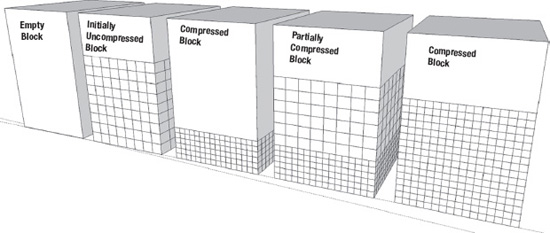
Figure 3-6. The OLTP compression process for non-direct path loads

The progression of states moves from left to right. Rows are initially loaded in an uncompressed state. As the block fills to the point where no more rows can be inserted, the row data in the block is compressed. The block is then placed back on the freelist and is capable of accepting more uncompressed rows. This means that in an OLTP-compressed table, blocks can be in various states of compression. All rows can be compressed, some rows can be compressed, or no rows can be compressed. This is exactly how records in HCC blocks behave when they are updated. A couple of examples will demonstrate this behavior. The first will show how the size of a table can balloon with updates.

This output shows that updating all the records in an HCC ARCHIVE LOW table expanded it to a slightly larger footprint than an OLTP-compressed (via direct path load) version of the same table. Interestingly enough, the update statement spent most of its time waiting on BUFFER BUSY WAITS. Apparently there is not a specific wait event for when a process is waiting while a block is being compressed. Here is the complete set of events that the update statement waited on (from a 10046 trace file processed with tkprof), along with per-second session statistics (both from one of the parallel slave processes):

The second example demonstrates that a row is migrated from an HCC block when it is updated. Basically we’ll update a single row, see that its rowid has changed, verify that we can still get to the record via its original rowid, and check to see if the TABLE FETCH CONTINUED ROW statistic gets updated when we access the row via its original rowid.

So the row has definitely been migrated. Now let’s verify that the migrated row is not compressed. We can do this by dumping the block where the newly migrated record resides. But before we look at the migrated row let’s have a look at the original block.

Now let’s look at the trace file produced in the trace directory. Here is an excerpt from the block dump.

The block is not compressed and conforms to the normal Oracle block format. Notice that there is only one row in the block (nrows=1). Also notice that the data_object_id is included in the block in hex format (seg/obj: 0x13081). The table has five columns. The values are displayed, also in hex format. Just to verify that we have the right block, we can translate the data_object_id and the value of the first column as follows:

As you can see, this is the record that we updated in the SKEW_HCC3 table. Just as an aside, it is interesting to see how the compressed block format differs from the standard uncompressed format. Here is a snippet from the original block in our example that is compressed for ARCHIVE LOW.

Notice that this block shows that it is compressed at level 3 (ARCHIVE LOW). Also notice that one record has been deleted from this block (migrated would be a more accurate term, as this is the record that we updated earlier). The line that says deleted rows: actually shows a list of the rows that have been migrated. Remember that we updated the record with rowid 7.3171084.0, meaning file 7, block 3171084, slot 0. So this line tells us that the one deleted row was in slot 0.

Expected Compression Ratios

HCC can provide very impressive compression ratios. The marketing material has claimed 10× compression ratios and believe it or not, this is actually a very achievable number for many datasets. Of course the amount of compression depends heavily on the data and which of the four algorithms is applied. The best way to determine what kind of compression can be achieved on your dataset is to test it. Oracle also provides a utility (often referred to as the Compression Advisor) to compress a sample of data from a table in order to calculate an estimated compression ratio. This utility can even be used on non-Exadata platforms as long as they are running 11.2.0.2 or later. This section will provide some insight into the Compression Advisor and provide compression ratios on some sample real world datasets.

Compression Advisor

If you don’t have access to an Exadata but still want to test the effectiveness of HCC, you can use the Compression Advisor functionality that is provided in the DBMS_COMPRESSION package. The GET_COMPRESSION_RATIO procedure actually enables you to compress a sample of rows from a specified table. This is not an estimate of how much compression might happen; the sample rows are inserted into a temporary table. Then a compressed version of that temporary table is created. The ratio returned is a comparison between the sizes of the compressed version and the uncompressed version. As of Oracle Database version 11.2.0.2, this procedure may be used on a non-Exadata platform to estimate compression ratios for various levels of HCC as well as OLTP compression. The Advisor does not work on non-Exadata platforms running Database versions prior to 11.2.0.2, although there may be a patch available to enable this functionality.

The Compression Advisor may also be useful on Exadata platforms. Of course you could just compress a table with the various levels to see how well it compresses, but if the tables are very large this may not be practical. In this case you may be tempted to create a temporary table by selecting the records where rownum < X and do your compression test on that subset of rows. And that’s basically what the Advisor does, although it is a little smarter about the set of records it chooses. Here’s an example of its use:

Notice that the procedure prints out a validation message telling you how many records were used for the comparison. This number can be modified as part of the call to the procedure if so desired. The get_compression_ratio.sql script prompts for a table and a Compression Type and then executes the DBMS_COMPRESSION.GET_COMPRESSION_RATIO procedure. Once again the pertinent data is a little hard to pick out of the listing, so Table 3-5 compares the actual compression ratios to the estimates provided by the Compression Advisor.

The estimates are fairly close to the actual values and while they are not 100 percent accurate, the tradeoff is probably worth it in cases where the objects are very large and a full test would be too time-consuming or take up too much disk space. The ability to run the Compression Advisor on non-Exadata platforms is also a real plus. It should be able to provide you with enough information to make reasonable decisions prior to actually migrating data to Exadata.

Real World Examples

As Yogi Berra once said, you can learn a lot just by watching. Marketing slides and book author claims are one thing, but real data is often more useful. Just to give you an idea of what kind of compression is reasonable to expect, here are a few comparisons of data from different industries. The data should provide you with an idea of the potential compression ratios that can be achieved by Hybrid Columnar Compression.

Custom Application Data

This dataset came from a custom application that tracks the movement of assets. The table is very narrow, consisting of only 12 columns. The table has close to 1 billion rows, but many of the columns have a very low number of distinct values (NDV). That means that the same values are repeated many times. This table is a prime candidate for compression. Here are the basic table statistics and the compression ratios achieved:

As expected, this table is extremely compressible. Simple queries against these tables also run much faster against the compressed tables, as you can see in this listing:

This simple query ran roughly 19 times faster using the ARCHIVE LOW compressed table than when it was run against the uncompressed table.

Telecom Call Detail Data

This table contains call detail records for a telecom company. There are approximately 1.5 billion records in the table. Many of the columns in this table are unique or nearly so. In addition, many of the columns contain large numbers of nulls. Nulls are not compressible since they are not stored in the normal Oracle block format. This is not a table we would expect to be highly compressible. Here are the basic table statistics and the compression ratios:

Financial Data

The next table is made up of financial data, revenue accrual data from an order entry system to be exact. Here are the basic table statistics.

So the number of rows is not that great, only about 115 million, but the table is wide. It has 161 columns and the average row length is 917 bytes. It is a bit of a mixed bag with regards to compressibility though. Many of the columns contain a high percentage of nulls. On the other hand, many of the columns have a very low number of distinct values. This table may be a candidate for reordering the data on disk as a strategy to improve the compression ratio. At any rate, here are the compression rates achieved on this table at the various HCC levels.

Retail Sales Data

The final table is made up of sales figures from a retailer. The table contains about 6 billion records and occupies well over half a Terabyte. There are very few columns, and the data is highly repetitive. In fact, there are no unique fields in this table. This is a very good candidate for compression. Here are the basic table statistics:

Here are the compression ratios achieved for this table. As expected they are very good.

Summary of the Real World Examples

The examples in this section came from real applications. They show a fairly extreme variation in data compressibility. This is to be expected, as the success of compression algorithms is very dependent on the data being compressed. Table 3-6 presents the data from all four examples.

Hopefully this data gives you some feel for the range of compression ratios that you can expect from HCC and the types of datasets that will benefit most. Of course the best way to predict how compressible a particular table may be is to actually test it. This fact cannot be overemphasized.

Restrictions/Challenges

There are a few challenges with using HCC. Many of them have to do with the fact that HCC is not available on non-Exadata platforms. This fact poses challenges for recovery and high availability solutions. The other major challenge is that HCC doesn’t play well with data that is being actively updated. In particular, systems characterized by lots of single-row updates, which we often describe as OLTP workloads, will probably not work well with HCC.

Moving Data to a non-Exadata Platform

Probably the largest hurdle with using HCC has been moving the data to non-Exadata platforms. For example, while RMAN and Dataguard both support the HCC block format, and will happily restore data to a non-Exadata environment, a database running on such an environment will not be able to do anything with the data until it is decompressed. This can mean a lengthy delay before being able to access the data in a case where a failover to a standby on a non-Exadata platform occurs. The same issue holds true for doing an RMAN restore to a non-Exadata platform. The restore will work but the data in HCC formatted blocks will not be accessible until the data has been moved into a non-HCC format. This can be done with the ALTER TABLE MOVE NOCOMPRESS command, by the way.

In addition to the lengthy delay associated with decompressing data before being able to access it, there is also the issue of space. If HCC is providing a 10× compression factor, you will need to have 10 times the space you are currently using available on the target environment to handle the increased size of the data. For these reasons, Dataguard is rarely set up with a standby on a non-Exadata platform.

Disabling Serial Direct Path Reads

As we discussed in Chapter 2, Serial Direct Path Reads allow nonparallelized scan operations to use the direct path read mechanism, which is a prerequisite for enabling the Smart Scan features of Exadata. Serial Direct Path Reads are enabled based on a calculation that depends on the size of the object being scanned relative to the available buffer cache. In simplistic terms, only large objects will be considered for Serial Direct Path Reads. HCC’s effectiveness can actually work against it here. Since the compression reduces the size of the objects so drastically, it can cause statements that would normally benefit from a Smart Scan to use the standard read mechanism, disabling many of Exadata’s optimizations. This is generally not a huge problem, because the number of blocks is considerably reduced by HCC and the database is making this decision at run time. The problem comes in, though, when an object is partitioned. The calculation is based on the size of the object being scanned; in the case of a partitioned object this means the size of the partition. So in cases where partitioning is used with HCC, we often see some partitions using Smart Scans and some unable to use Smart Scans. Keep in mind that this also means decompression cannot be done at the storage layer, as this capability is enabled only when performing Smart Scans.

Locking Issues

The Exadata documentation says that updating a single row of a table compressed with HCC locks the entire compression unit containing the row. This can cause extreme contention issues for OLTP-type systems. This is the main reason that HCC is not recommended for tables (or partitions) where the data will be updated. Here’s a demonstration of the locking behavior:

Clearly this behavior would be disastrous to many OLTP systems. Especially when you consider the large number of records that can be stored in an HCC block. In this case that number is approximately 13,500 rows per block. This means that a single update could lock well over 50,000 rows.

Single Row Access

HCC is built for full table scan access. Decompression is a CPU-intensive task. Smart Scans can distribute the decompression work to the CPU’s on the storage cells. This makes the CPU-intensive task much more palatable. However, Smart Scans only occur when Full Scans are performed. This means that other access mechanisms, index access for example, must use the DB server CPUs to perform decompression. This can put an enormous CPU load on DB servers in high volume OLTP-type systems. In addition, since data for a single row is spread across multiple blocks in a CU, retrieving a complete row causes the entire CU to be read. This can have a detrimental effect on the overall database efficiency for systems that tend to access data using indexes, even if the access is read-only.

Common Usage Scenarios

HCC provides such high levels of compression that it has been used as an alternative to traditional ILM strategies, which generally involve moving older historical data off the database entirely. These ILM strategies usually entail some type of date range partitioning and a purge process. This is done to free storage and in some cases to improve performance. Often the data must be retained in some backup format so that it can be accessed if required at some later date. With HCC, it is possible in many cases to retain data indefinitely by compressing the oldest partitions. This approach has many advantages over the traditional approach of moving the data.

First and foremost, the data remains available via the standard application interfaces. No additional work will need to be done to restore a backup of old data before it can be accessed. This advantage alone is often enough to justify this approach. This approach typically entails leaving active partitions uncompressed while compressing old partitions more aggressively. Here’s a short example of creating a partitioned table with mixed compression modes.

Summary

Introduced in Oracle 11g R2, Hybrid Columnar Compression provides exceptional compression capabilities that are far beyond anything available in prior releases. This is thanks in large part to the adoption of industry-standard compression algorithms and an increase in the size of the compression unit from a single database block (typically 8K) to a larger unit of 32K or 64K. The feature is only appropriate for data that is no longer being modified, though, because of locking issues and the fact that updated rows are moved into a much less compressed format (OLTP compression format). For this reason, HCC should only be used with data that is no longer being modified (or only occasionally modified). Since compression can be defined at the partition level, it is common to see tables that have a mixture of compressed and uncompressed partitions. This technique can in many cases replace ILM approaches that require moving data to alternate storage media and then purging it from the database.