C H A P T E R  7

Resource Management

If resources were unlimited, there would be no need to manage them. We see this in all aspects of our daily lives. If yours was the only car on the road, traffic signals wouldn't be necessary. If you were the only customer at the bank, there would be no need for the winding ropes that form orderly lines. But as we all know, this is rarely the case. It is the same for database servers. When the load on the system is light, there is very little need for resource management. Processes complete in a fairly consistent period of time. But when the system gets busy and resources become scarce, we can find ourselves with an angry mob on our hands.

For a number of years now, Oracle's Database Resource Manager (DBRM) has provided an effective way to manage the allocation of critical resources within the database. Without DBRM, all database connections are treated with equal priority, and they are serviced in a sort of round-robin fashion by the operating system scheduler. When the system is under heavy load, all sessions are impacted equally. Low-priority applications receive just as high a priority as business-critical applications. It is not uncommon to see a few poorly written ad-hoc queries degrade the performance of mission-critical applications. If you've been a DBA long enough, especially in data warehouse environments, you're probably familiar with the Unix renice command. It is a root-level command that allows you to influence the CPU priority of a process at the operating-system level. A number of years ago, we worked in a DBA group supporting a particularly heavily loaded data warehouse. The renice command was used frequently to throttle back CPU priority for database sessions that were dominating the system. There were a couple of obvious problems with this approach. First of all, it was a privileged command available only to the root user, and system administrators were reluctant to grant DBAs access to it. The second problem was that automating it to manage CPU resources was difficult at best. Oracle's Database Resource Manager is a much more elegant solution to the problem. It allows DBAs to address resource allocation within the domain of the database itself. It is a well-organized, framework that is automated by design. It ensures that critical system resources like CPU and I/O will be available to your important applications whenever they are needed, even when the system is under a heavy workload. This is done by creating resource allocation schemes that define priorities based on the needs of the business.

Another case for resource management is consolidation. It was inevitable that a platform with the performance, capacity, and scalability of Exadata would be viewed by many as an ideal consolidation platform. But consolidating databases is a challenge, mainly because of the difficulty of managing resources across databases. We've worked with a number of clients who have used Exadata to consolidate multiple database servers onto the Exadata platform. One such client consolidated 29 databases from 17 database servers onto two Exadata full racks. Needless to say, without Oracle's resource management capabilities, it would be extremely difficult, if not impossible, to balance system resources among so many database environments. Until recently there was really no way to prioritize I/O across databases. With Exadata V2, Oracle introduced I/O Resource Manager (IORM), and for the first time we can virtually guarantee I/O service levels within and among databases.

So whether you are consolidating multiple databases onto your Exadata platform or handling resource intensive applications within a single database, effective resource management will play an important role in your success. In this chapter we will review and demonstrate the main components of DBRM and how it is used to manage and allocate CPU resources effectively within a database. We'll also take a look at instance caging and how it can be used to set limits on the amount of CPU a database may use in order to provide predictable service levels for multi-tenant database environments. In the last half of the chapter we'll cover the new Exadata-specific feature called I/O Resource Manager, which allocates and prioritizes disk I/O at the storage cell.

Oracle Resource Manager, for all its benefits, has been an infrequently used feature of the database. This is largely due to its complexity and a general lack of understanding among the DBA community. Beyond introducing the new Exadata-specific features of Resource Manager, our goals in presenting this material are twofold. First we want to provide enough detail to demystify Oracle Resource Manager without overwhelming the reader. Second, we intend to demonstrate how to build a fully functional resource management model. These goals present a unique challenge. Provide too little information, and the reader will only be able to set up very simple configurations. Too much detail, and we risk convoluting the topic and losing the audience. The most difficult part of writing this chapter has been striking a balance between the two. As you read through the examples you will notice that we used multi-level resource plans. This is not to suggest that in order to be effective, you must use complex multi-level plans. In fact, simple, single-level resource plans will solve a vast majority of the resource management problems we see in the real world. Moreover, multi-level resource plans can be difficult to design and test. In this chapter we demonstrate multi-level plans because it is important to understand how they work. But if you are considering using Oracle Resource Manager, the best approach is to keep it simple, and add features only as they are needed.

Database Resource Manager

Database Resource Manager (DBRM) has been around for a number of years and is basically geared toward managing CPU resources and I/O (indirectly) at the database tier. Exadata V2 introduced a new feature called I/O Resource Manager (IORM), which, as you might expect, is geared toward managing and prioritizing I/O at the storage cell. When databases on Exadata request I/O from the storage cells, they send additional information along with the request that identifies the database making the request as well as the consumer group making the request. The software on the storage cells (Cellserv or cellsrv) knows about the priorities you establish inside the database (DBRM) and/or at the Storage Cell (IORM), and it manages how I/O is scheduled. DBRM and IORM are tightly knit together, so it is important to have a solid understanding of DBRM before IORM is going to make any sense to you. Now, Database Resource Manager is a lengthy topic and could easily justify a book all by itself. So here, we'll focus on the basic constructs that we will need for constructing an effective IORM Resource Plan. If you already have experience with DBRM, you may be able to skip over this topic, but be aware that the examples in this section will be used as we discuss IORM in the last half of the chapter.

Before we begin, let's review the terminology that will be used in this topic. Table 7-1 describes the various components of Database Resource Manager. We'll discuss these in more detail as we go along.

As shown in the table, DBRM consists of three main components: resource consumer groups (consumer groups), resource plan directives (plan directives), and resource plans.

Consumer groups: A consumer group can represent a single database session or a group of sessions. Generally speaking, consumer groups consist of end users or application groups that share a common business priority. Grouping sessions together in this manner allow resources to be assigned and managed collectively. For example, in a mixed-workload database environment, consumer group assignments allow you to collectively assign more CPU and I/O resources to your high-priority business applications while reducing the resources allocated to low-priority applications.

Plan directives: Plan directives are where you define your resource allocations. A plan directive is created using the CREATE_PLAN_DIRECTIVE procedure. In addition to defining the resource allocation itself (percentage of CPU, for example), the procedure also requires you to name one resource plan and one consumer group. In this way, a plan directive “links,” or assigns a consumer group to a resource plan. Only one consumer group may be assigned to a directive, and resource plans typically consist of multiple directives. you can say that a consumer group is assigned to a resource plan through the creation of a plan directive.

Resource plan: The resource plan is the collection of directives that determine how and where resources are allocated. Only one plan may be activated in the database instance at any given time. The resource plan is activated by assigning it to the RESOURCE_MANAGER_PLAN instance parameter. For example, the following alter system command activates the resource plan ‘myplan':

SQL> alter system set resource_manager_plan=’myplan’;

A database's resource plan may be changed at any time, allowing you to reallocate resources at various times of the day, week, or month in order to meet the varying workload requirements of your business. When the resource plan is activated, no resources are allocated to individual user sessions. Instead, resources are allocated to the consumer groups according to the directives in the resource plan.

Consumer Groups

When a resource plan is activated, DBRM examines key attributes of all sessions in the database and assigns them to consumer groups. Sessions are assigned to consumer groups by means of mapping rules that you define. For example, a set of user accounts can be mapped to a consumer group based on their user name or the machine from which they are logging in. A user may belong to many different consumer groups and may be dynamically reassigned from one consumer group to another even in the middle of executing a SQL statement or query. Since database resources are allocated only to consumer groups, reassigning a session to another group immediately changes its resource allocation. All sessions in a consumer group share the resources of that group. For example, if the APPS consumer group is allocated 70% of the total CPU on the server, all sessions belonging to that consumer group will equally share the 70% allocation of CPU. There are two built-in consumer groups in every database: syS_GROUP and OTHER_GROUPS. These groups cannot be modified or dropped.

syS_GROUP: This is the default consumer group for the syS and sySTEM user accounts. These accounts may be assigned to another consumer group using mapping rules we'll discuss in the next section.

OTHER_GROUPS: This is the default consumer group. Any sessions that belong to a consumer group that is not defined in the currently active resource plan will automatically be mapped to this consumer group. This is Oracle's way of making sure all user sessions are assigned to a consumer group in the active resource plan.

Consumer Group Mapping Rules

All user sessions (except syS and sySTEM) are mapped by default to the consumer group OTHER_GROUPS. This behavior can be modified using mapping rules so that sessions are automatically reassigned to other consumer groups. If there is no mapping rule for a session, or if the mapping rules assign the session to a consumer group that is not named in the currently active plan, then it will be automatically assigned to this built-in consumer group. Every resource plan must have the OTHER_GROUPS resource group to handle this condition. The following example shows how a mapping rule is created. This mapping rule calls for the TPODER account to be automatically assigned to the REPORTS consumer group, while anyone logging in using the Payroll.exe application will be mapped to the APPS consumer group:

There are two types of session attributes that can be used to create mapping rules: login attributes and runtime attributes. Login attributes are set when the user logs in and do not change during the life of the session. Resource Manager uses login attributes to determine which consumer group the session should initially be assigned to. Runtime attributes are set at runtime and can be changed at any time during the life of the session by the client application. Table 7-2 describes the session attributes Resource Manager can use for creating session-to-consumer-group mapping rules.

Conflicts can occur between mapping rules when a user account matches more than one rule. Oracle resolves these conflicts by allowing you to specify the relative priority of each attribute. This way, Oracle can automatically determine which rule (attribute) should take precedence when session attributes satisfy multiple mapping rules. The default priorities for the ORACLE_USER and CLIENT_APPLICATION attributes are 6 and 7, respectively. In the following example, I've promoted the CLIENT_PROGRAM to position 2, and the ORACLE_USER to position 3. Now the client application establishing a database connection will take precedence over the client's USERNAME.

For example, using the mapping rules and priorities we've created so far, let's say TPODER logs in to the database. According to the ORACLE_USER mapping rule, this user would ordinarily be assigned to the REPORTS consumer group. But if TPODER logs in from the company's Payroll application, his session will be mapped to the APPS consumer group. This is because according to the rule priorities, the CLIENT_APPLICATION mapping rule takes precedence over ORACLE_USER. The following query shows how two different sessions from the same user account get mapped according to the username and client program mapping priorities. Notice how only the Payroll application, payroll.exe, overrides the REPORTS mapping rule.

Plan Directives

DBRM allocates database resources to consumer groups through plan directives. A plan directive consists of one consumer group and one or more management attributes. There is a one-to-one relationship between a plan directive and a consumer group, and no two directives may be assigned to the same resource group (within the same plan). A plan directive is made up of a list of management attributes in a key=value fashion. For example, the following listing shows how a set of directives may be defined in DBRM:

MGMT_Pn

Exadata's IO Resource Manager works with DBRM through plan directives using the CPU management attributes MGMT_Pn, (where n may be 1–8), and MAX_UTILIZATION_LIMIT, so going forward these attributes will be the focus our discussion. CPU is allocated in a level + percentage manner. Usage of the MGMT_Pn attribute determines the relative priority in which CPU is allocated to consumer groups across the various levels, where 1 is the highest level/priority. The percentage assigned to the MGMT_Pn attribute determines how available CPU resources (unallocated plus unused) are allocated within a particular level. Whatever CPU is unused or unallocated from level 1 is allocated to level 2. Unused and unallocated CPU from level 2 is then passed to the consumer groups on level 3. If there are two consumer groups on level 2 and one of them doesn't use its allocation, the unused CPU is always passed to the next level in the Plan. The other consumer group on level 2 can't utilize it.

Figure 7-1 shows a simple resource plan and illustrates how this level + percentage method of allocating CPU resources works.

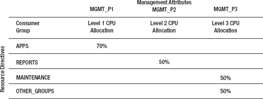
Figure 7-1. Resource directives

In Figure 7-1 the APPS group is allocated 70% of total CPU available to the database. Sessions in the REPORTS group are the next highest priority at level 2 and will be allocated half of the unallocated CPU (30%) from level 1. Sessions in the resource groups MAINTENANCE and OTHER_GROUPS equally share unallocated CPU (50%) from level 2. This can be expressed in formula form as follows:

APPS = 70%                           (100% × 70%)

REPORTS = 15%                    ((100% – 70%) × 50%)

MAINTENANCE = 7.5%          (((100%  70%) × 50%) × 50%)

OTHER_GROUPS = 7.5%        (((100%  70%) × 50%) × 50%)

Resource Manager is designed to maximize CPU utilization. This is important to understand because it means that there are times when consumer groups may actually exceed their allocation. When CPU resources are limited, plan directives define guaranteed service levels for consumer groups. But when extra CPU is available, plan directives also determine how unused CPU resources are allocated among consumer groups. For example, if CPU utilization in the APPS group falls below 70%, half of the unused CPU is redistributed to the REPORTS group on level 2 (mgmt._p2=50%), and half is distributed to the consumer groups on level 3. If the REPORTS group does not fully utilize its allocation of CPU, the unused CPU is also redistributed to the consumer groups on level 3. If you need to set an absolute limit on CPU for a consumer group, use the MAX_UTILIZATION_LIMIT directive.

Resource Plan

A resource plan is a collection of plan directives that determine how database resources are to be allocated. you may create any number of resource plans for your database that allow you to meet the specific service levels of your business, but only one may be active at any given time. you may deactivate the current resource plan and activate another plan whenever the needs of the business change. When the active resource plan changes, all current and future sessions will be allocated resources based on directives in the new plan. Switching between various resource plans is commonly done to provide suitable allocations for particular times of the day, week, or month. For example, an after-hours plan may be activated in the evening to favor database backups, batch jobs, extracts, and data-loading activities. Other applications for maintaining multiple plans may include month-end processing, year-end processing, and the like.

The Pending Area

Resource plans in the database cannot be directly modified; nor can you directly define new plan directives or resource groups. Oracle provides a work space called the pending area for creating and modifying all the elements of a resource plan. you can think of it as a loading zone where all the elements of your resource plan are staged and validated together before they are submitted to DBRM. There may be only one pending area in the database at any given time. If a pending area is already open when you try to create one, Oracle will display the error message, “ORA-29370: pending area is already active.” The pending area is not a permanent fixture in the database. you must explicitly create it before you can create or modify resource plans. The following listing shows the typical process of creating a pending area, validating your changes, and then submitting it. After the pending area is submitted, it is automatically removed and a new one must be created if you want to perform any additional work on DBRM components. The following listing shows how the Pending Area is created, validated, and submitted.

Resource Manager Views

Oracle supplies a number of views that report configuration, history, and metrics for Resource Manager. Let's take a look at a few of the views that are useful for reviewing and monitoring resources in your DBRM configuration.

V$RSRC_CONSUMER_GROUP: The V$RSRC_CONSUMER_GROUP view displays information about the active resource consumer groups. It also contains performance metrics that are useful for tuning purposes. We'll take a closer look at this view when we test a resource plan later on in the chapter.

V$RSRC_PLAN: This view displays the configuration of the currently active resource plan.

V$RSRC_PLAN_HISTORy: The V$RSRC_PLAN_HISTORy view shows historical information for your resource plans, including when they were activated and deactivated, and whether they were enabled by the database scheduler or scheduler windows.

V$RSRC_SESSION_INFO: This view shows performance statistics for sessions and how they were affected by the Resource Manager.

V$SESSION: The V$SESSION view is not specifically a Resource Manager view but its RESOURCE_CONSUMER_GROUP field is useful for determining what resource group a session is assigned to.

DBA_RSRC_CATEGORIES: This view displays the resource categories that are configured in the database. Categories are used by the I/O Resource Manager for controlling storage cell I/O allocation within a database.

DBA_RSRC_CONSUMER_GROUPS: This view displays all the consumer groups defined in the database.

DBA_RSRC_CONSUMER_GROUP_PRIVS: This view reports users, and the resource groups to which they have been granted permission. A user must have permission to switch to a consumer group before the session-to-consumer group mapping rules will work.

DBA_RSRC_GROUP_MAPPINGS: This view lists all the various session-to-resource group mapping rules defined in the database.

DBA_RSRC_MAPPING_PRIORITy: This view reports the priority of session attributes used in resolving overlaps between mapping rules.

DBA_RSRC_IO_CALIBRATE: This view displays the I/O performance metrics DBRM uses for I/O resource management. Maximum read rates are captured for I/O operations per second (IOPS), megabytes per second (MBPS), and latencies for data block read requests.

DBA_RSRC_PLANS: This view lists all resource plans and the number of plan directives assigned to each plan in the database.

DBA_RSRC_PLAN_DIRECTIVES: This view lists all resource plan directives, resource allocation percentages, and levels defined in the database.

DBA_USERS: This view is not actually a Resource Manager view but it does display the username and initial resource group assignment, in its INITIAL_RSRC_CONSUMER_GROUP field.

DBA_HIST_RSRC_CONSUMER_GROUP: This view displays historical performance metrics for Resource consumer groups. It contains AWR snapshots of the V$RSRC_CONS_GROUP_HISTORy view.

DBA_HIST_RSRC_PLAN: This is a simple view that displays historical information about resource plans such as when they were activated and deactivated.

The Wait Event: resmgr: cpu quantum

DBRM allocates CPU resources by maintaining an execution queue similar to the way the operating system's scheduler queues processes for their turn on the CPU. The time a session spends waiting in this execution queue is assigned the wait event resmgr: cpu quantum. A CPU quantum is the unit of CPU time (fraction of CPU) that Resource Manager uses for allocating CPU to consumer groups. This event occurs when Resource Manager is enabled and is actively throttling CPU consumption. Increasing the CPU allocation for a session's consumer group will reduce the occurrence of this wait event and increase the amount of CPU time allocated to all sessions in that group. For example, the CPU quantum wait events may be reduced for the APPS resource group (currently 70% at level 1) by increasing the group's CPU allocation to 80%.

DBRM Example

Now that we've discussed the key components of DBRM and how it works, let's take a look at an example of creating and utilizing resource plans. In this example we'll create two resource plans similar to the one in Figure 7-1. One allocates CPU resources suitably for critical DAyTIME processing, and the other favors night-time processing.

Step 1: Create Resource Groups

The first thing we'll do is create the resource groups for our plan. The following listing creates three resource groups, APPS, REPORTS, and MAINTENANCE. Once we have the resource groups created, we'll be able to map user sessions to them.

Step 2: Create Consumer Group Mapping Rules

Okay, so that takes care of our resource groups. Now we'll create our session-to-resource group mappings. The following PL/SQL block creates mappings for three user accounts (KOSBORNE, TPODER, and RJOHNSON), and just for good measure, we'll create a mapping for our TOAD users out there. This will also allow us to see how attribute mapping priorities work.

One more important step is to grant each of these users permission to switch their session to the consumer group you specified in your mapping rules. If you don't, they will not be able to switch their session to the desired resource group and will instead be assigned to the default consumer group, OTHER_GROUPS. So if you find that user sessions are landing in OTHER_GROUPS instead of the resource group specified in your mapping rules, you probably forgot to grant the switch_consumer_group privilege to the user. Remember that this will also happen if the mapping rule assigns a session to a consumer group that is not in the active resource plan. The GRANT_OPITON parameter in the next listing determines whether or not the user will be allowed to grant others permission to switch to the consumer group.

Step 3: Set Resource Group Mapping Priorities

Since we want to use more than the session's USERNAME to map sessions to resource groups, we'll need to set priorities for the mapping rules. This tells DBRM which rules should take precedence when a session matches more than one rule. The following PL/SQL block sets a priority for the client program attribute higher than that of the database user account:

Step 4: Create the Resource Plan and Plan Directives

Generally speaking, resource plans are created at the same time as the plan directives. This is because we cannot create an empty plan. A resource plan must have at least one plan directive, for the OTHER_GROUPS resource group. The following listing creates a resource plan called DAyTIME and defines directives for the resource groups: APPS, REPORTS, MAINTENANCE, and, of course, OTHER_GROUPS.

Step 5: Create the Night-Time Plan

Organizations typically have different scheduling priorities for after-hours work. The NIGHTTIME plan shifts CPU allocation away from the APPS resource group to the MAINTENANCE group. The next listing creates the NIGHTTIME plan with priorities that favor maintenance processing over applications and reporting. Even so, 50% of CPU resources are reserved for the APPS and REPORTS resource groups to ensure that business applications and reports get sufficient CPU during off-peak hours.

Step 6: Activate the Resource Plan

Once our resource plans are created, one of them must be activated for DBRM to start managing resources. Resource plans are activated by setting the instance parameter RESOURCE_MANAGER_PLAN, using the ALTER sySTEM command. If the plan doesn't exist, then DBRM is not enabled.

you can automatically set the activate resource plan using scheduler windows. This method ensures that business rules for resource management are enforced consistently. The following listing modifies the built-in scheduler window WEEKNIGHT_WINDOW so that it enables our nighttime resource plan. The window starts at 6:00 PM (hour 18) and runs through 7:00 AM (780 minutes).

Now we'll create a new window that covers normal business hours, called WEEKDAy_WINDOW. This window will automatically switch the active resource plan to our DAyTIME resource plan. The window starts at 7:00 AM (hour 7) and runs until 6:00 PM (660 minutes), at which point our WEEKNIGHT_WINDOW begins.

Testing a Resource Plan

Before we finish with Database Resource Manager, let's test one of our resource plans to see if it works as advertised. Validating the precise CPU allocation to each of our resource groups is a very complicated undertaking, so we won't be digging into it too deeply. But we will take a look at the V$RSRC_CONSUMER_GROUP view to see if we can account for how the CPU resources were allocated among our consumer groups. For the test, we'll use the SCRATCH database, and the DAyTIME resource plan we created earlier. The results of the test will:

• Verify that sessions map properly to their Resource Groups
• Show how to identify DBRM wait events in a session trace
• Verify that CPU is allocated according to our resource plan

Figure 7-2 shows resource allocation directives for the DAyTIME resource plan we'll be testing.

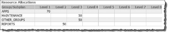
Figure 7-2. DAyTIME resource plan allocation

If our DAyTIME resource plan is working, CPU will be allocated according to the following formula. Note that the 70%, 15%, 7.5%, and 7.5% allocations reflect the percent of total CPU.

Level 1) APPS = 70%                      (100% × 70%)

Level 2) REPORTS = 15%               ((100% - 70%) × 50%)

Level 3) MAINTENANCE = 7.5%      (((100% - 70%) × 50%) × 50%)

Level 3) OTHER_GROUPS = 7.5%     (((100% - 70%) × 50%) × 50%)

Test Outline

Now that we've created our resource plan, we can test to see how it works. Following are the steps we will follow to test our resource plan.

1. Turn off the Database Resource Manager.
2. Start a session using the RJOHNSON account.
3. Start 20 concurrent CPU intensive queries from each of the user accounts that map to our consumer groups. These user accounts map to resource groups as follows:
   KOSBORNE        APPS
RJOHNSON        REPORTS
TPODER      MAINTENANCE
FRED        OTHER_GROUPS
4. Check the consumer group assignments in the V$SESSION. RESOURCE_CONSUMER_GROUP view. This column should be null, since DBRM is inactive.
5. Start a 10046 session trace on an RJOHNSON session.
6. Run a CPU intensive query from the RJOHNSON session.
7. Tail the session trace file and watch for resmgr:cpu quantum wait events. There shouldn't be any at this point, because DBRM is inactive.
8. While the load test is still running, activate the DAyTIME resource plan.
9. Check the consumer group assignments again. Now that DBRM is active, sessions should be assigned to their respective consumer groups.
10. Check the RJOHNSON session trace file again. We should see resmgr:cpu quantum wait events now that the DAyTIME resource plan is active.
11. Review the Resource Manager metrics in the V$RSRC_CONSUMER_GROUP view to see how CPU resources were allocated during the test. We should see CPU allocated according to the directives in our resource plan.

Step 1: Deactivate DBRM

Now, we'll begin our test of the resource plan. The first thing we'll do is turn off DBRM by setting the instance database parameter RESOURCE_MANAGER_PLAN to '' (an empty string).

Step 2: Log In as RJOHNSON

Now, we'll start a SQL*Plus session, logging in as RJOHNSON.

Step 3: Start Load Test

In four separate terminal windows, we'll generate a load on the system by running a shell script that spins up 20 SQL*Plus sessions for each user account. Each session kicks off the following query, which creates a Cartesian product. The skew table has 32,000,000 rows, so the join will create billions of logical I/O operations. That, along with the sum on COL1, should create sufficient CPU load for our tests. The following listing shows the definition of the SKEW table, with indexes on the COL1 and COL2 columns.

Now, let's start the test queries and take a look at the CPU utilization. The following listing shows the query we'll be using for the test.

The burn_cpu.sh shell script, shown next, executes 20 concurrent copies of the burn_cpu.sql script. We'll run this script once for each of the user accounts, FRED, KOSBORNE, RJOHNSON, and TPODER. Our test configuration is a single database (SCRATCH), on a quarter rack Exadata V2. Recall that the V2 is configured with two quad-core CPUs.

With DBRM disabled, our test sessions put a heavy load on the CPU. Output from the top command shows 26 running processes and user CPU time at 80.8%:

Step 4: Check Consumer Group Assignments

Let's take a look at our session-to-consumer group mappings. When DBRM is inactive, sessions will show no consumer group assignment. This is another way to verify that Resource Manager is not active.

The query output shows a total of 81 sessions, consisting of twenty sessions per user account, plus one interactive RJOHNSON session that we'll trace in the next step. No sessions are currently mapped to the resource groups, because DBRM is inactive.

Step 5: Start 10046 Session Trace for the interactive RJOHNSON session

Now we'll start a 10046 trace for the interactive RJOHNSON session so we can see the Resource Manager wait events that would indicate DBRM is actively regulating CPU for this session. Remember that DBRM is still inactive, so we shouldn't see any Resource Manager wait events in the trace file yet.

Step 6: Execute a Query from the RJOHNSON Session

Next, we'll execute a long-running, CPU-intensive query, from the interactive RJOHNSON session. This is the same query we used for the load test in Step 3.

Step 7: Examine the Session Trace File

Since our resource plan is not active yet, we don't see any Resource Manager wait events in the trace file at this point.

Step 8: Activate Resource Manager

Now, while the load test is still running, let's enable DBRM by setting the active resource plan to our DAyTIME plan. When the resource plan is activated, our resource mapping rules should engage and switch the running sessions to their respective consumer groups.

Step 9: Check Consumer Group Assignments

Now, let's run that query again and see what our consumer group assignments look like.

Our user sessions are mapping perfectly. The query shows that all user sessions have been switched to their consumer group according to the mapping rules we defined earlier.

Step 10: Examine the Session Trace File

Now, let's take another look at the session trace we started in step 2 and watch for DBRM wait events (resmgr:cpu quantum). The output from the trace file shows the wait events Oracle used to account for the time our interactive RJOHNSON session spent in the DBRM execution queue, waiting for its turn on the CPU:

As you can see, the RJOHNSON user session is being given a limited amount of time on the CPU. The ela= attrbute in the trace records shows the amount of time (in microseconds) that the session spent in the resmgr:cpu quantum wait event. In the snippet from the trace file, we see that the RJOHNSON session was forced to wait for a total of 266,786 microseconds, or .267 CPU seconds. Note that the output shown here represents a very small sample of the trace file. There were actually thousands of occurrences of the wait event in the trace file. The sum of the ela time in these wait events represents the amount of time the session was forced off the CPU in order to enforce the allocation directives in the DAyTIME plan.

Step 11: Check DBRM Metrics

And finally, if we look at the V$RSRC_CONSUMER_GROUP view, we can see the various metrics that Oracle provides for monitoring DBRM. These counters are reset when a new resource plan is activated. Some accumulate over the life of the active plan, while others are expressed as a percentage and represent a current reading.

Table 7-3 shows the definitions of the CPU-related columns we're interested in.

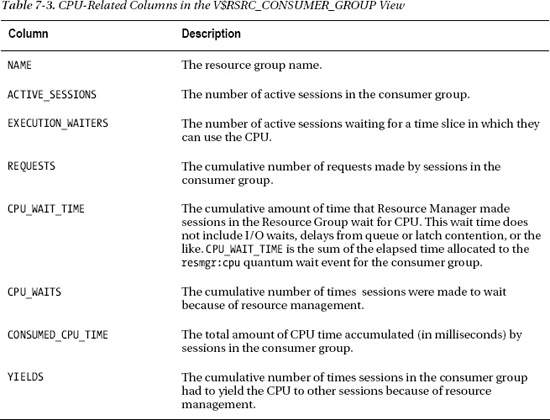
The following listing is a report you may use to display the metrics collected in the V$RSRC_CONSUMER_GROUP view. These metrics are a valuable tool for determining the effect our resource allocations had on the consumer groups during the test.

In this report you can see how Resource Manager allocated CPU resources to the consumer groups according to our plan directives. Notice the BACKGROUND resource group (named_ORACLE_BACKGROUND_GROUP_). Database background processes are assigned to this special group. Processes included in this group include pmon, smon, dbw, lgwr, and a host of other familiar background processes that manage the database. Assigning performance-critical processes to this group is the way Resource Manager excludes them from resource management. For all other consumer groups, you can see that Resource Manager forced sessions to yield the processor in order to distribute CPU resources according to our resource directives. The number of yields and CPU waits are of interest, but not as telling as the CPU wait time and CPU time consumed. The percentages in Figure 7-3 show how CPU and wait time were allocated among our consumer groups.

Figure 7-3. DAyTIME resource plan allocation

According to Resource Manager, the APPS group consumed 68.48% of the total CPU used by foreground processes, which is very close to the 70% we allocated it in our resource plan. At 15.33%, the REPORTS group was almost a perfect match to the 15% our plan called for. The MAINTENANCE group used 8.23%, which was a little high but still a very good fit with the 7.5% we defined for it. The OTHER_GROUPS used 7.63% CPU, which again was nearly a perfect match with our plan directive of 7.5%. We should mention that at first the allocations in this report were not proportioned very closely to the allocations in our resource plan. We had to let the stress test run for several minutes before DBRM was able to get the numbers fine-tuned to the levels we see in Figure 7-3.

In conclusion, even though the test results show minor variances between CPU allocated in our plan directives and CPU utilization reported, you can see that DBRM was, in fact, managing CPU resources according to our plan. The test also verified that user sessions properly switched to their respective consumer groups according to our mapping rules when the resource plan was activated.

Database Resource Manager has been available for a number of years now. It is a very elegant, complex, and effective tool for managing the server resources that are the very life blood of your databases. Unfortunately, in our experience, it is rarely used. There are probably several reasons for this. DBAs are continually barraged by complaints that queries run too long and applications seem sluggish. We are often reluctant to implement anything that will slow anyone down. This is often compounded when multiple organizations within the company share the same database or server. It is a difficult task to address priorities within a company where it comes to database performance; and the decision is usually out of the control of DBAs, who are responsible for somehow pleasing everyone. Sound familiar? Our suggestion would be to start small. Separate the most obvious groups within your database by priority. Prioritizing ad-hoc queries from OLTP applications would be a good place to start. With each step you will learn what works and doesn't work for your business. So start small. Keep it simple, and implement resource management in small, incremental steps.

Instance Caging

While Resource Manager plan directives provision CPU usage by consumer group within the database, instance caging provisions CPU at the database instance level. Without instance caging, the operating system takes sole responsibility for scheduling processes to run on the CPUs according to its own algorithms. Foreground and background processes among all databases instances are scheduled on the CPUs without respect to business priorities. Without instance caging, sessions from one database can monopolize CPU resources during peak processing periods and degrade performance of other databases on the server. Conversely, processes running when the load on the system is very light tend to perform dramatically better, creating wide swings in response time from one moment to the next. Instance caging allows you to dynamically set an absolute limit on the amount of CPU a database may use. And because instance caging enforces a maximum limit on the CPU available to the instance, it tends to smooth out those wide performance swings and provide much more consistent response times to end users. This is not to say that instance caging locks the database processes down on a specific set of physical CPU cores (a technique called CPU affinity); all CPU cores are still utilized by all database background and foreground processes. Rather, instance caging regulates the amount of CPU time (% of CPU) a database may use at any given time.

Instance caging also solves several less obvious problems caused by CPU starvation. Some instance processes are critical to overall health and performance of the Oracle database. For example, if the log writer process (LGWR) doesn't get enough time on the processor, the database can suffer dramatic, system-wide brownouts because all database write activity comes to a screeching a halt while LGWR writes critical recovery information to the online redo logs. Insufficient CPU resources can cause significant performance problems and stability issues if Process Monitor (PMON) cannot get enough time on the CPU. For RAC systems, the Lock Management Server (LMS) process can even cause sporadic node evictions due to CPU starvation, (we've seen this one a number of times).

Instance caging directly addresses CPU provisioning for multitenant database environments, making it a very useful tool for database consolidation efforts. For example, let's say you have four databases, each running on a separate server. These servers each have four outdated CPUs, so consolidating them onto a new server with 16 brand-new CPU cores should easily provide performance that is at least on par with what they currently have. When you migrate the first database, the end users are ecstatic. Queries that used to run for an hour begin completing in less than 15 minutes. you move the second database, and performance slows down a bit but is still much better than it was on the old server. The queries now complete in a little less than 30 minutes. As you proceed to migrate the remaining two databases, performance declines even further. To aggravate the situation, you now find yourself with mixed workloads all competing for the same CPU resources during peak periods of the day. This is a common theme in database consolidation projects. Performance starts off great, but declines to a point where you wonder if you've made a big mistake bringing several databases together under the same roof. And even if overall performance is better than it was before, the perception of the first clients to be migrated is that it is actually worse, especially during peak periods of the day. If you had used instance caging to set the CPU limit for each database to four cores when they were moved, response times would have been much more stable.

Configuring and Testing Instance Caging

Configuring instance caging is very simple. Activating a resource plan and setting the number of CPU cores are all that is required. Recall that the active resource plan is set using the database parameter RESOURCE_PLAN. The number of CPUs is set using the CPU_COUNT parameter, which determines the number of CPUs the instance may use for all foreground and background processes. Both parameters are dynamic, so adjustments can be made at any time. In fact, scheduling these changes to occur automatically is a very useful way to adjust database priorities at various times of the day or week according to the needs of your business. For example, month-end and year-end processing are critical times for accounting systems. If your database server is being shared by multiple databases, allocating additional processing power to your financial database during heavy processing cycles might make a lot of sense.

Now, let's take a look at instance caging in action. For this example we'll use our SCRATCH and SNIFF databases to demonstrate how it works. These are standalone (non-RAC) databases running on an Exadata V2 database server with two quad core CPUs. The Nehalem chipset is hyper-threaded, so the database actually “sees” 16 virtual cores (or CPU threads), as you can see in the following listing.

We'll be using the built-in resource plan, DEFAULT_PLAN, for these tests. Figure 7-4 shows the CPU resource allocation for this plan. Note that under the default_plan, all users other than syS and sySTEM will be mapped to the OTHER_GROUPS resource group.

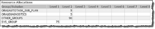
Figure 7-4. DEFAULT_PLAN resource allocation

For this test, we'll use the same script we used for testing our DBRM resource plans in the previous section. Again, the burn_cpu.sh script with a parameter of 20 will spin up 20 concurrent sessions, each running the test query. This should drive the CPU utilization up to approximately 80%. Once the sessions are running, we'll use the top command to see the effect instance caging has on the server CPU load. Let's start out by getting a baseline. To do this, we'll run the test with instance caging and Resource Manager turned off. Recall that these tests are running on a quarter rack Exadata V2, which is configured with two quad-core hyper-threaded CPUs. So the database instances see a CPU_COUNT of 16.

As you can see, running the burn_cpu.sh script drove the CPU usage up from a relatively idle 0.3%, to 82.9%, with 25 running processes. Now, let's see what happens when we reset the cpu_count to 8, which is 50% of the total CPU on the server. Notice that the number of running processes has dropped from 25 to 10. The CPU time in user space has dropped to 46.1%, just over half of what it was.

Now, we'll set the CPU_COUNT parameter to 4. That is half of the previous setting, so we should see the CPU utilization drop by about 50%. After that, we'll drop the CPU_COUNT to 1 to illustrate the dramatic effect instance caging has on database CPU utilization. Notice that when we set the number of CPUs to 4, our utilization dropped from 46% to 25%. Finally, setting CPU_COUNT to 1 further reduces CPU utilization to 4.8%.

This test illustrated the effect of instance caging on a single database. Now let's configure two databases and see how instance caging controls CPU resources when multiple databases are involved.

In the next two tests we'll add another database to the mix. The SNIFF database is identical to the SCRATCH database we used in the previous test. In the first of the next two tests, we'll run a baseline with instance caging turned off by setting CPU_COUNT set to 16 in both databases. The baseline will run 16 concurrent copies of the test query on each database. We'll let it run for a few minutes and then take a look at the CPU utilization of these databases as well as the readings from the top command. The active resource plan for both databases is set to DEFAULT_PLAN, and CPU_COUNT is set to 16.

Figure 7-5 shows a summary of our second test. Each line, representing a session foreground process, shows the percentage of one CPU core. This is summed and divided by 16 (CPU cores) to get the percentage of total CPU consumed. As expected, the distribution of CPU between our two databases is approximately equal at 44.6% and 45.3%. Looking at the Total Connection CPU, we can see that the databases accounted for about 90% of total CPU time for the server.

Figure 7-5. Test summary: two databases, instance caging turned off

The source for the data reflected in this summary was collected as follows:

% of 1 Core: Individual process CPU from the %CPU column from the top command.

% of Total CPU: Result of % of 1 Core / 16 cores (CPU threads).

User: Cpu(s): nn.nn%us from the top command.

Kernel: Cpu(s): nn.nn%sy from the top command.

Idle: Cpu(s): nn.nn%id from the top command.

Total CPU: Sum of User, Kernel, and Idle.

Total Connection CPU: Sum of % of Total CPU for each database.

Total Other + Idle CPU: Total CPU – Total Connection CPU.

SCRATCH %: % of Total CPU(SCRATCH) / Total Connection CPU.

SNIFF %: % of Total CPU(SNIFF) / Total Connection CPU.

The ‘SCRATCH %', and ‘SNIFF %' numbers are what we're interested in. They represent the percentage of total CPU used by all sessions in each of these databases. As you can see from the summary, the databases were split at approximately 50% each.

Now let's run the same load test with instance caging configured for a 75/25 split on the number of cores assigned to SCRATCH and SNIFF respectively. In this test, SCRATCH gets 12 CPUs (75% of 16 cores), and SNIFF gets 4 CPUs (25% of 16 cores).

Figure 7-6 shows the results of our second test. The split isn't perfect. It is closer to an 80/20 split. Not captured in these tests was the amount of CPU consumed by all the database background processes, so that may account for the some of the difference. It is also important to understand that Oracle's Resource Manager operates in the user space of the O/S process model, rather than the kernel space. So it cannot directly control the amount of CPU a process consumes inside the kernel; it can only influence this by throttling processes in the user space. In our summary, we see that the SCRATCH database sessions consumed 78.79% of total session CPU, while the SNIFF database used 21.21% of total session CPU. Even though the split isn't perfect, it does show that instance caging made a solid effort to manage these databases to the 75/25 split we defined. Now, this is not to say that instance caging locks the database processes down on a specific set of physical CPU cores. All CPU cores are still utilized by all database background and foreground processes. Rather, instance caging regulates the amount of CPU time (% of CPU) a database may use at any given time.

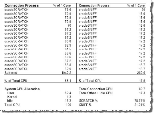
Figure 7-6. Test summary: two databases, instance caging, 75% / 25% split

Over-Provisioning

Over-provisioning refers to the practice of allocating more CPUs to the databases than are actually installed in the server. This is useful when your server hosts multiple databases with complementing workload schedules. For example, if all the heavy processing for the SCRATCH database occurs at night, and the SNIFF database is only busy during DAyTIME hours, it wouldn't make sense to artificially limit these databases to 8 CPU threads each (8×8). A better CPU allocation scheme might be more on the order of 12×12. This would allow each database to fully utilize 12 cores during busy periods, while still “reserving” 4 cores for off-peak processing by the other database. DBAs who consolidate multiple databases onto a single server are aware that their databases don't use their full CPU allocation (CPU_COUNT) all of the time. Over-provisioning allows unused CPU to be utilized by other databases rather than sitting idle. Over-provisioning has become a popular way of managing CPU resources in mixed workload environments. Obviously, over-provisioning CPU introduces the risk of saturating CPU resources. Keep this in mind if you are considering this technique. Be sure you understand the workload schedules of each database when determining the most beneficial CPU count for each database.

Instance caging limits the number of CPU cores a database may use at any given time, allowing DBAs to allocate CPU to databases based on the needs and priorities of the business. It does this through the use of the instance parameter CPU_COUNT. Our preference would have been to allocate CPU based on a percentage of CPU rather the number of cores. This would give the DBA much finer-grained control over CPU resources and would be especially useful for server environments that support numerous databases. But CPU_COUNT is tightly coupled with Oracle's Cost Based Optimizer (CBO), which uses the number of CPUs for its internal costing algorithms. It wouldn't make sense to allow the DBA to set the percentage of processing power without matching that with the value the CBO uses for selecting optimal execution plans. It probably would have been a much more difficult effort to implement such a change to the optimizer. Be that as it may, instance caging is a powerful new feature that we've been waiting for, for a long time and is a major advancement database resource management.

I/O Resource Manager

Earlier in this chapter we discussed Oracle's Database Resource Manager, which manages CPU resources within a database through consumer groups and plan directives. Sessions are assigned to resource groups, and plan directives manage the allocation of resources by assigning values such as CPU percentage to resource management attributes such as MGMT_P1..8. DBRM, however, is limited to managing resources within the database.

DBRM manages I/O resources in a somewhat indirect manner by limiting CPU and parallelism available to user sessions (through consumer groups). This is because until Exadata came along, Oracle had no presence at the storage tier. Exadata lifts I/O Resource Management above the database tier and manages I/O at the storage cell in a very direct way. Databases installed on Exadata send I/O requests to cellsrv on the storage cells using a proprietary protocol known as Intelligent Database protocol (iDB). Using iDB, the database packs additional attributes in every I/O call to the storage cells. This additional information is used in a number of ways. For example, IORM uses the type of file (redo, undo, datafile, control file, and so on) for which the I/O was requested to determine whether caching the blocks in flash cache would be beneficial or not. Three other attributes embedded in the I/O request identify the database, the consumer group, and the consumer group's category. These three small bits of additional information are invaluable to Oracle's intelligent storage. Knowing which database is making the request allows IORM to prioritize I/O requests by database. Categories extend the concept of consumer groups on Exadata platforms. Categories are assigned to consumer groups within the database using Database Resource Manager. Common categories, defined in multiple databases, can then be allocated a shared I/O priority. For example, you may have several databases that map user sessions to an INTERACTIVE category. I/O requests coming from the INTERACTIVE category may now be prioritized over other categories such as REPORTS, BATCH, or MAINTENANCE.

IORM provides three distinct methods for I/O resource management: Interdatabase, Category, and Intradatabase. These methods may be used individually or in combination. Figure 7-7 illustrates the relationship of these three I/O resource management methods.

Figure 7-7. Three methods for I/O resource management

Interdatabase IORM (Interdatabase Resource Plan): IORM determines the priority of an I/O request based on the name of the database initiating the request. Interdatabase IORM is useful when Exadata is hosting multiple databases and you need to manage I/O priorities among the databases.

IORM Categories (Category Resource Plan): IORM determines the priority of an I/O request among multiple databases by the category that initiated the request. Managing I/O by category is useful when you want to manage I/O priorities by workload type. For example, you can create categories like APPS, BATCH, REPORTS, MAINTENANCE in each of your databases and then set an I/O allocation for these categories according to their importance to your business. If the APPS category is allocated 70%, then sessions assigned to the APPS category in all databases share this allocation.

Intradatabase IORM (Intradatabase Resource Plan): Unlike Interdatabase and Category IORM, Intradatabase IORM is configured at the database tier using DBRM. DBRM has been enhanced to work in partnership with IORM to provide fine-grained I/O resource management among resource groups within the database. This is done by allocating I/O percentage and priority to consumer groups using the same mechanism used to allocate CPU, the MGMT_Pn attribute. For example, the SALES database may be allocated 50% using Interdatabase IORM. That 50% may be further distributed to the APPS, REPORTS, BATCH, and OTHER_GROUPS consumer groups within the database. This ensures that I/O resources are available for critical applications, and it prevents misbehaving or I/O-intensive processes from stealing I/O from higher-priority sessions inside the database.

How IORM Works

IORM manages I/O at the storage cell by organizing incoming I/O requests into queues according the database name, category, or consumer group that initiated the request. It then services these queues according to the priority defined for them in the resource plan. IORM only actively manages I/O requests when needed. When a cell disk is not fully utilized, cellsrv issues I/O requests to it immediately. But when a disk is heavily utilized, cellsrv instead redirects the I/O requests to the appropriate IORM queues and schedules I/O from there to the cell disk queues according to the policies defined in your IORM plans. For example, using our SCRATCH and SNIFF databases from earlier in this chapter, we could define a 75% I/O directive for the SCRATCH database, and a 25% I/O directive for the SNIFF database. When the storage cells have excess capacity available, the I/O queues will be serviced in a first-in-first-out (FIFO) manner. During off-peak hours, the storage cells will provide maximum throughput to all databases in an even-handed manner. But when the storage cell begins to saturate, the SCRATCH queue will be scheduled 75% of the time, and the SNIFF queue will be scheduled 25% of the time. I/O requests from database background processes are scheduled according to their relative priority to the foreground processes (client sessions). For example, while the database writer processes (DBWn) are given priority equal to that of foreground processes, performance critical I/O requests from background processes that maintain control files, and redo log files are given higher priority.

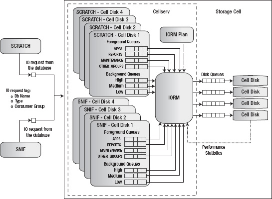
IORM Architecture

Figure 7-8 illustrates the architecture of IORM. For each cell disk, cellsrv (Cellserv) maintains an IORM queue for each consumer group, and each background process (high, medium, and low priority), for each database accessing the storage cell. By managing the flow of I/O requests between the IORM queues and the disk queues, cellsrv provides very effective I/O prioritization at the storage cells. I/O requests sent to the storage cell include tags that identify the database and the consumer group issuing the request, as well as the type of I/O (redo, control file, and so on). For databases that do not have an Intradatabase resource plan defined, foreground processes are automatically mapped to the consumer group OTHER_GROUPS. Three separate queues are maintained for background processes so that cellsrv may prioritize scheduling according to the type of I/O request. For example, redo and control file I/O operations are sent to the high-priority queue for background processes. IORM schedules I/O requests from the consumer group queues according to the I/O directives in your IORM Plan.

Figure 7-8. IORM architecture

Limiting Excess I/O Utilization

Ordinarily, when excess I/O resources are available (allocated but unused by other consumer groups), IORM allows a consumer group to use more than its allocation. For example if the SCRATCH database is allocated 60% at level 1, it may consume I/O resources above that limit if other databases have not fully utilized their allocation. you may choose to override this behavior by setting an absolute limit on the I/O resources allocated to specific databases. This provides more predictable I/O performance for multi-tenant database server environments. The LIMIT IORM attribute is used to set a cap on the I/O resources a database may use even when excess I/O capacity is available. The following listing shows an IORM plan that caps the SCRATCH database at 80%.

By the way, maximum I/O limits may also be defined at the consumer group level, by using the MAX_UTILIZATION_LIMIT attribute in your DBRM resource plans.

Workload Optimization

To optimize I/O performance, IORM distinguishes between small and large I/O requests. Requests less than 128K in size, typically associated with OLTP transactions, are categorized as small (SM) requests. Requests 128K in size or greater, which are generally associated with DW transactions, are categorized as large (LG) requests. The distinction between small and large I/O requests is important because the algorithms used for optimizing low-latency I/O requests (small requests) and high-throughput I/O requests (large requests) are polar opposites. For OLTP transactions, low latency is most important. For example, consider an end user waiting for a quick ZIP code search to populate the screen. To provide optimized performance for low-latency requests, large I/O requests must be managed in such a way that they don't fully consume the I/O resources of the storage cell. Conversely, DW transactions require high throughput to maximize performance. To optimize I/O for throughput, the storage cell must service many concurrent large I/O requests so that it is fully consumed. By comparing the large (LG) and small (SM) I/O requests in the IORM metrics, you can determine whether your databases lean more toward a DW workload or an OLTP workload. Recently, Oracle added a new attribute to IORM, known as the optimization objective. This attribute determines the optimization mode IORM will use when managing cell disk I/O queues. The optional values for the IORM objective attribute are as follows:

low_latency: This setting provides optimization for applications that are extremely sensitive to I/O latency. It provides the lowest possible I/O latencies, by significantly limiting disk utilization. In other words, throughput-hungry applications will be significantly (negatively) impacted by this optimization objective.

high_throughput: This setting provides the best possible throughput for DW transactions, by attempting to fully utilize the I/O capacity of the storage cells. It is the opposite of low_latency and as such, it will significantly (negatively) impact disk I/O latency.

Balanced: This setting attempts to strike a balance between low latency and high throughput. This is done by limiting disk utilization for large I/O operations to a lesser degree than the low_latency objective described above. Use this objective when workloads are mixed and you have no applications that require extremely low latency.

Auto: This setting allows IORM to determine the best optimization objective for your workload. Cellsrv continuously monitors the large/small I/O requests and applies the optimization method on a best-fit basis. If 75% or more of the I/O operations from a consumer group are small I/O (less than 128K), then it is considered to be a latency-oriented consumer group and is managed accordingly.

The default setting for an IORM plan objective is ‘' (an empty string). The objective may be set using the CellCLI alter iormplan objective objective command as follows:

Methods for Managing I/O on Exadata

As introduced earlier, there are three methods for managing I/O on the Exadata platform: Interdatabase IORM, Category IORM, and Intradatabase IORM. All three address specific needs for managing I/O. Interdatabase IORM allocates I/O resources by database name, Category IORM allocates I/O resources by common categories among databases, and Intradatabase IORM manages I/O within the database using DBRM resource groups. you can choose to use any one of the methods for managing your I/O resources, or you combine them to implement a more sophisticated resource plan. When these methods are used together, Oracle schedules I/O in the following order: 1) allocation among categories, 2) allocation among databases, and 3) allocation among consumer groups within each category within each database. We'll show how all this works a little later.

Interdatabase I/O Resource Management

Interdatabase I/O resource management refers to the IORM feature that manages I/O priority among multiple databases by database name. Interdatabase IORM allocates I/O resources across multiple databases by means of an IORM plan configured on each storage cell. The IORM plan defines allocation priorities using I/O directives. Each storage cell manages its own I/O queues based on the local IORM plan defined in the cell. IORM plans should be identical for all storage cells in the storage grid. If you have split your Exadata storage cells into multiple storage grids, then IORM plans may differ from grid to grid, but they should still be identical among storage cell members within each storage grid. We discuss configuring multiple storage grids in Chapter 14. Figure 7-9 illustrates how I/O allocation policies are organized within the IORM plan.

Figure 7-9. Interdatabase IORM plan

In Figure 7-9, our SCRATCH database, the highest-priority database, is guaranteed 60% of the total I/O on level 1. On level 2, our SNIFF database takes its 80% slice of the remaining 40% of unallocated I/O from level 1. Any unused I/O from level 1 also cascades down to level 2. In addition to any unconsumed I/O from levels 1 and 2, databases on level 3 will equally share the unallocated 16% of total I/O, (16% = 80% × 20%). Note that any databases that do not explicitly appear in the active I/O resource plan will automatically be assigned to the OTHER group.

Configuring Interdatabase IORM

Interdatabase I/O Resource Manager is configured using an IORM plan. This plan determines the database I/O priorities for the storage cell. IORM plans are created using the CellCLI command ALTER IORMPLAN. There can be only one IORM plan per storage cell, regardless of how many ASM instances (clustered or single instance) use it for storage. Creating an Interdatabase IORM plan is fairly simple. The first step is to determine what your allocation policy should be for each database. you will use these allocation policies to define the directives for your IORM plan. The LEVEL attribute specifies the priority a database should be given relative to other databases in the plan. The ALLOCATION attribute determines the percentage of I/O a database will be given out of the total I/O available on its level. The following example demonstrates how you to create an IORM plan to implement the allocation policies illustrated in Figure 7-9.

The CellCLI command list iormplan detail displays our new IORM plan. Notice that the catPlan attribute is empty. This is a placeholder for the Category IORM plan we'll be looking in the next topic.

The aggregate allocation for all databases on a level may not exceed 100%. If the sum of allocations on any level exceeds 100%, CellCLI will throw an error. For example, the following listing shows the error CellCLI produces when over 100% is allocated on level 1:

Before our Interdatabase IORM Plan can manage I/O resources, it must be activated using the CellCLI command ALTER IORMPLAN ACTIVE. For now, we'll leave it turned off. Later, in the “Understanding IORM Metrics” section of the chapter, we'll test our Interdatabase IORM Plan and discuss how the effects of IORM can be monitored at the storage cells.

Category IORM

The I/O Resource Manager (IORM) extends the concept of resource groups with a new attribute known as a category. While resource groups allow DBRM to manage resources within a database, categories provide I/O resource management among multiple databases. For example, suppose our two databases (SCRATCH and SNIFF) have similar workloads. They both host OLTP applications that do short, time-sensitive transactions. During business hours, these transactions must take priority. These databases also do a fair amount of batch processing, such as running reports and maintenance jobs. The batch processing takes a lower priority during business hours. These two workloads can be managed and prioritized using IORM categories. The categories APPS_CATEGORy and BATCH_CATEGORy can be defined in both databases for high-priority applications and long-running, lower-priority activities, respectively. If APPS_CATEGORy is allocated 70% on level 1, then no matter how heavily loaded the storage grid is, sessions assigned to this category, for both databases, will be guaranteed a minimum of 70% of all I/O.

Configuring Category IORM

Setting up Category IORM is fairly straightforward. Once you've created your DBRM consumer groups, you will create categories in the database and assign them to your consumer groups. The final step is to create an IORM plan in the storage cells to establish I/O allocation and priority for each category. you can define as many as eight levels in your Category IORM Plan. Figure 7-10 illustrates the relationship between consumer groups, categories, and the Category IORM Plan.

Figure 7-10. IORM resource management by category

For this exercise, we'll create two new categories, APPS_CATEGORy, and BATCH_CATEGORy, and assign them to the APPS, REPORTS, and MAINTENANCE resource groups we created earlier in the chapter. The following listing creates our new categories and assigns them to the resource groups. Remember that you will need to run these commands on all databases participating in the IORM Category Plan. For illustration purposes, we'll keep the number of categories to two. The REPORTS and MAINTENANCE resource groups will be assigned to the category BATCH_CATEGORy.

To check your resource-group-to-category mappings, query the DBA_RSRC_CONSUMER_GROUPS view as follows. Notice that the OTHER_GROUPS consumer group was assigned to the OTHER category. That mapping is created automatically by Oracle and cannot be altered.

Now we can create a new Category IORM Plan on the storage cells and set I/O limits on these categories. Before we do, though, we'll drop the Interdatabase IORM Plan we created in the previous example. Remember that each storage cell maintains its own IORM plan, so you will need to run these commands on every cell in your storage grid.

Now we're ready to create our Category IORM Plan. The following command creates a plan in which APPS_CATEGORy and BATCH_CATEGORy are allocated 70% and 30%, respectively, of the total Cell I/O at level 1. The default category, OTHER, is allocated 100% on level 2.

Again, we'll use the CellCLI command list iorm detail and confirm that our Category IORM Plan is configured the way we want it:

Because we dropped the Interdatabase plan from the previous exercise, the dbPlan field is empty. We'll reinstall that plan again when we are ready to test our resource plans. Note that the IORM Plan is inactive. We'll leave our Category Plan inactive for now. Later, in the IORM metrics section of the chapter, we'll test our Category IORM Plan and discuss how the effects of IORM can be monitored at the storage cells.

Intradatabase IORM

In the case of Interdatabase I/O resource management, cellsrv identifies I/O requests by a tag containing the database name issuing the request. Category I/O resource management works in a similar way, using a tag in the I/O request to identify the category issuing the request. The third, and final, type of I/O resource management available on the Exadata platform is Intradatabase IORM. Intradatabase I/O resource management is configured in each database using DBRM's management attributes, MGMT_P1..8. you may recall from earlier in the chapter that the MGMT_Pn attributes are what DBRM uses to manage CPU resources. DBRM uses CPU allocation directives to define priorities among consumer groups within the database. By tying I/O allocations to CPU allocations, IORM carries forward these priorities to the storage layer, thus maintaining a consistent provisioning scheme for both.

Configuring Intradatabase IORM

Intradatabase IORM is not terribly difficult to implement. In fact, in a manner of speaking, we have already done so. In the DBRM section of this chapter, we created consumer groups, resource plans, and plan directives that managed CPU resources within the SCRATCH database. On the Exadata platform, when a DBRM resource plan is activated, the database transmits a description of the plan, including MGMT_Pn directives, to all cells in the storage grid. This also happens any time cellsrv is started on the storage cells. So whether you're installing a new cell into the storage grid, rebooting a cell, or bouncing cellsrv services, your Intradatabase resource plan will be pushed to the cell automatically. If IORM is active on the cell, it will generate an Intradatabase Plan and begin managing I/O priorities according to your resource directives. Figure 7-11 illustrates the process of configuring and activating Intradatabase IORM.

Figure 7-11. An Intradatabase I/O resource plan

In Figure 7-11, we see the calls to DBMS_RESOURCE_MANAGER that created our resource plan and plan directives for the SCRATCH and SNIFF databases. These directives are used to assign CPU and I/O allocation for the resource groups APPS, REPORTS, MAINTENANCE, and OTHER_GROUPS. When the DAyTIME plan is activated, its definition is sent to cellsrv on the storage cells. When cellsrv receives the resource plan, it generates an Intradatabase IORM Plan, configures I/O queues for each consumer group, and begins to manage I/O resources.

Bringing It All Together

As discussed earlier, each of the three IORM management methods may be used individually or in combination. Let's take a look at how all three methods work together to manage I/O. Now, this is the part where your college accounting professor would say “each lesson builds on the last, so if you skipped class last week, you may feel a little lost today.” In this exercise, we'll be using all of the elements of DBRM and IORM we've discussed in this chapter. To avoid confusion and save you the trouble of thumbing through the pages you've already read, Table 7-4 shows a summary of how we've configured Oracle Resource Manager for the SCRATCH and SNIFF databases in this chapter.

There is a fixed order of precedence between the three IORM methods we've discussed. As I/O requests traverse the layers of the IORM stack, they are divided and allocated by the next method. At the top of the IORM hierarchy, 100% of I/O resources are available because the storage cell is not saturated by I/O requests. The next level of the hierarchy is Category IORM, which allocates I/O at a 70/30 split between the categories APPS_CATEGORy and BATCH_CATEGORy (at level 1). Any unconsumed I/O between these two groups is available to the OTHER category at level 2.

Next in the IORM hierarchy is the Interdatabase Plan. At the database level, the 70% allocated to the APPS_CATEGORy category is further divided, giving 60% to the SCRATCH database on level 1, and 80% to the SNIFF database at level 2. Any other database receives 20% of the unallocated I/O from level 2, as well as access to any I/O that was not consumed by the SCRATCH and SNIFF databases on levels 1 and 2.

The third and final tier of the IORM hierarchy is Intradatabase IORM. Our Intradatabase plan further divides I/O allocation into the four DBRM consumer groups we created in the databases. The APPS consumer group gets top priority at 70% on level 1. The REPORTS group is allocated 50% at level 2. MAINTENANCE and OTHER_GROUPS share a 50/50 split of I/O that was unallocated or unconsumed at levels 1 and 2.

Now, this is not to imply that all resource management methods must be configured together. you may instead choose to use just one of the methods, or any combination of two, for managing I/O. For example if we had configured Category IORM alone then as illustrated in Figure 7-12, no further restriction of I/O resources would be performed. I/O resources would be split at 70/30 between the categories, APPS_CATEGORy and BATCH_CATEGORy. Similarly, you may choose to implement Interdatabase IORM by itself, in which case I/O will be allocated strictly at a 60/80 split between sessions in the SCRATCH and SNIFF databases, respectively. If you have only one database and need to manage differing workloads, then Intradatabase IORM is your only option. When Intradatabase IORM is used by itself, I/O is managed according to your DBRM Plan directives alone. Figure 7-12 shows how I/O calls are allocated as they filter through each layer of IORM.

Figure 7-12. IORM method heirarchy

In Figure 7-12, allocations for the default consumer group OTHER_GROUPS and the default category OTHER are not shown, because of space constraints. In Figures 7-13, 14, and 15 we see the calculations used to allocate I/O resources as shown in Figure 7-12. The OTHER_GROUPS consumer group and OTHER category are shown here along with their allocation. Figures 7-13 through 7-15 shows a tabular representation of the resource plans along with their allocation percentage. Also displayed in these examples are the formulas used to calculate the allocation.

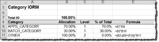
Figure 7-13. Category IORM calculations

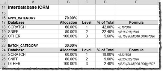
Figure 7-14. Interdatabase IORM calculations

Figure 7-15. Intradatabase IORM calculations

IORM Monitoring and Metrics

I/O performance metrics are collected and maintained for IORM in the storage cell. These metrics may be used to determine the effects your IORM plan has on the databases, categories, and resource group resource directives you defined in your environment. For example, you can see how much I/O a particular database is using compared to other databases. By observing the actual I/O distribution for your IORM consumer groups, you can determine whether adjustments need to be made to provide adequate I/O resources for applications using your databases. In this section we'll look at how these metrics are organized and tap into the valuable information stored there.

Understanding IORM Metrics

When an IORM plan is defined in the storage cell, cellsrv creates I/O consumer groups corresponding to the I/O directives defined in the Intradatabase, Category, and Intradatabase IORM Plans. For example, the following I/O consumer groups were created in the storage cells from our IORM plan for the SCRATCH and SNIFF databases:

Interdatabase:  SCRATCH,

          SNIFF

          OTHER

Category:        APPS_CATEGORy

          BATCH_CATEGORy

          OTHER

Intradatabase: APPS

          REPORTS

          MAINTENANCE

          OTHER_GROUPS

Every 60 seconds, cellsrv collects key performance metrics from the I/O queues and stores them in the METRICCURRENT object. Note that we said object, not table or file. Cellsrv is a Java program, written by Java developers, not SQL developers. So unfortunately, these metrics are not stored in the familiar tabular format DBAs have come to know and love. Instead of tables, columns, and rows, these metrics are stored in objects and attributes. The following listing shows the structure of the METRICCURRENT object along with a few sample records.

When a new collection is run, the previous set of metrics is moved to the METRICHISTORy object, where it is kept for a period of time. Metric history is retained for the number of days specified in the METRICHISTORyDAyS attribute of cell, (the default is 7 days). For example, the next listing shows that cellsrv will maintain a rolling history of 7 days.

If you determine that 7 days is not sufficient history for your needs, you can modify the retention period with the CellCLI command alter cell. The following listing shows how you can change the retention for your storage cells to 14 days.

Workload Management

IORM metrics provide insight into how cellsrv is allocating I/O resources among the consumers in your storage grid. Cellsrv keeps track of I/O requests broadly categorized as “small requests” and “large requests.” By comparing the large (LG) and small (SM) I/O requests in the IORM metrics, you can determine whether your databases lean more toward a DW workload (high throughput) or an OLTP workload (low latency). Oracle recently added a new option to the IORM plan called objective that tells IORM to optimize the cell disk I/O queues for low latency, high throughput, or something in between. The IORM metric IORM_MODE was added to capture the objective in use during the collection period. By comparing the IORM_MODE with the actual workload on your storage cells, you can determine whether the current IORM objective is appropriate or not. For example, if you find that a majority of I/O operations in the storage cells are greater than 128K and thus large (LG), then IORM should be set to optimize for high throughput (objective=high_throughput). Oracle uses a threshold of 75% large I/O when the IORM objective is set to auto, so that should give you an idea of what is meant by “majority.” For more information on the IORM objective and possible settings, refer to the Workload Optimization section earlier in this chapter. The IORM_MODE metric can be observed using the following CellCLI command.

Possible settings for the IORM_MODE attribute are as follows:

• 1, IORM objective was set to low_latency,
• 2, IORM objective was set to balanced
• 3, IORM mode was set to high_throughput

An IORM_MODE ranging between 1 and 2, or between 2 and 3, indicates the mode was changed during the polling period. It also indicates the proximity to the IORM objective. This might occur, for example, if the objective was set to auto and during the polling period the workload shifted significantly from small I/O requests to large I/O requests. By comparing the IORM_MODE metric over time, you can determine how volatile your workload is. A constantly changing workload may give insight into where I/O Resource Management is needed the most.

The metrics we're interested in for IORM monitoring have an objectType of IORM_DATABASE , IORM_CATEGORy, and IORM_CONSUMER_GROUP. These metrics are further organized by the name attribute in the METRICCURRENT object. The name of the metric is a concatenation of abbreviations that indicate the type of I/O consumer group, the type of storage device, and a descriptive name. The elements of the name attribute appear as follows:

Where consumer_type represents the IORM resource group and is one of these:

DB = Interdatabase IORM Plan

CT = Category IORM Plan

CG = Intradatabase IORM Plan

And device_type is the type of storage that serviced the I/O request and is one of the following:

FC = flash cache

FD = Flash-based grid disk

‘’ = If neither of the above, then the metric represents I/O to physical disksy

The last part of the attribute, {metric}, is the descriptive name of the metric. The metric name may be further qualified by SM' or LG, indicating that it represents small I/O requests or large I/O requests. For example:

CG_FC_IO_RQ_LG: The total number of large I/O requests serviced from flash cache (FC), for DBRM consumer groups.

CG_FD_IO_RQ_LG: The total number of large I/O requests serviced from flash-based grid disks (FD), for DBRM consumer groups.

CG_IO_RQ_LG: The total number of large I/O requests serviced from physical disks (grid disks), for DBRM consumer groups.

Table 7-5 describes each of the IORM consumer group performance metrics captured by cellsrv using these abbreviations.

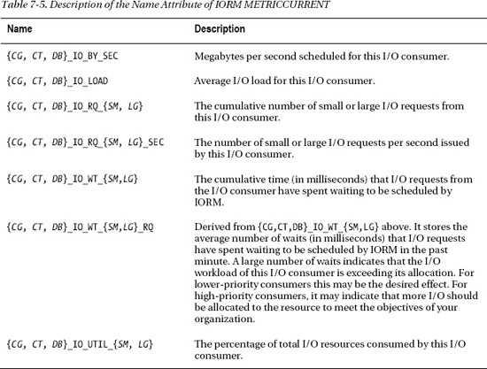
All cumulative metrics above are reset to 0 whenever cellsrv is restarted, the IORM plan is enabled, or the IORM plan changes for that I/O consumer group. For example, if the Category IORM plan is changed, the following cumulative metrics will be reset:

CT_IO_RQ_SM

CT_IO_RQ_LG

CT_IO_WT_SM

CT_IO_WT_LG

These IORM metrics are further categorized using the metricObjectName attribute. Interdatabase resource plan metrics for the SCRATCH, and SNIFF databases are stored in detail records, where metricObjectName is set to the corresponding database name. In a similar fashion, metrics for Category IORM Plans are identified with a metricObjectName matching the Category name. IORM consumer groups are identified by a concatenation of the database name and the name of the DBRM consumer group. For example, the following listing shows how the I/O Resource Groups for our SCRATCH and SNIFF databases would be represented in the METRICCURRENT and METRICHISTORy objects.

Background Processes

As we discussed earlier, database background processes are automatically assigned to built-in IORM consumer groups according to priority. Table 7-6 shows these special IORM consumer groups, along with a description of what they are used for.

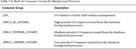
Mining the Metrics

Now that you have a pretty good idea of what types of metrics are collected by cellsrv, and how to get to them, let's take a look at how this information can be reported and interpreted. First, however, we should mention that as a reporting tool, CellCLI is very limited. For example, multiple filters can be applied to your search criteria using =, LIKE, or AND, but the lack of an OR verb, and the lack of parentheses for setting precedence, make it somewhat cumbersome; if not utterly inadequate for reporting. Also, there is no aggregation functionality. For example, there is no way to roll up the small and large I/O requests for a database and present them as “Total I/O Requests.” The long and short of it is, you are better off to just dump out all the rows you are interested in, load them into a database, and use SQL*Plus to report them. Now, let's take a look at some simple LIST commands for extracting IORM metrics along with a sample of the output they generate.

Reporting IORM Database Metrics

This first listing reports I/O metrics for our Database IORM Plan, (name like 'DB_IO_.*'). The objectType = ‘IORM_DATABASE' isn't really necessary; we've just included it to illustrate that this is the only objectType stored for this metric.y

Reporting IORM Category Metrics

To report I/O metrics for our Category Resource Plan, the name filter is changed to 'CT_IO_.*'. Adding an additional filter on the ObjectName metric (not like '_.*'), eliminates Oracle's automatically maintained categories such as _ASM_, and _ORACLE_BG_CATEGORY_.

Reporting IORM Consumer Group Metrics

To report I/O metrics for our consumer groups, we replace the name filter with CG_IO_.*, which displays I/O metrics for consumer groups. The additional filters for metricObjectName remove other databases from the output as well as consumer groups that Oracle creates for background processes, such as _ORACLE_BACKGROUND_GROUP_. The collectionTime was omitted from the sample output because of space constraints.

Testing IORM Plans

Earlier in the chapter, we postponed testing our IORM plans. Now that you understand how to monitor IORM, we can run a stress test and take a look at the metrics collected by cellsrv to see what effect our IORM plans had on performance. For this test, we'll generate a load on the storage cells by running several concurrent full-table scans on our SCRATCH and SNIFF databases. We'll let them run for a few minutes and then collect the database, category, and consumer group metrics for our test databases. As with our DBRM tests earlier in this chapter, validating the precise allocations for each I/O consumer is a very complicated undertaking, because any I/O resources that are allocated but unused are passed to other consumer groups, categories, and databases. This is particularly true when implementing multi-level resource plans. The focus of this test will be to verify that cellsrv is collecting metrics for each database, category, and consumer group, and that the relative I/O utilization numbers for each consumer group are within a reasonable range considering their resource allocations. Refer back to Figures 7-13 through 7-15 for the I/O allocations for each of our resource plans.

Test Outline

Now that we've created our I/O resource plan, we can test to see how it works. Following are the steps we will follow to test our resource plan.

1. Activate the DAYTIME resource plan in the SCRATCH and SNIFF databases. Also, activate the Database and Category IORM plans in each storage cell.
2. In both databases, start three concurrent full table scans from each account that maps to our consumer groups. These user accounts map to the consumer groups as follows:

   KOSBORNE       APPS

   RJOHNSON       REPORTS

   TPODER           MAINTENANCE

   FRED                OTHER_GROUPS

3. Allow the queries to run for a few minutes, and then, while they are still running, we'll dump the IORM metrics for database, category, and consumer groups to a file. This data will be cleaned up and loaded into an Oracle database for reporting.

Step 1: Activate Resource Manager

Before we start the load test, we need to verify that our DAYTIME resource plan is activated in the databases.

Step 2: Start Load Test

Next, we'll start our load test by running the burn_io.sh script in eight separate terminal sessions, one for each user account in the SCRATCH and SNIFF databases. This script is similar to the burn_cpu.sh script we used to test our DBRM resource plan earlier. The script takes three parameters: USERNAME, PASSWORD, and PARALLEL. The PARALLEL parameter determines how many queries will be run concurrently. For our test, we'll run three sessions from each user account. The query isy

The SQL script turns off output from the query, (set TERMOUT off) to reduce the overhead on the database server. The bigtab table contains 194 million (repeating) rows from the dba_segments view.

Step 3: Dump IORM Metrics to a File.

We'll allow the stress test to run for a while and then gather the IORM metrics from the storage cells. The following listing shows the CellCLI command for reporting IORM metrics. These metrics are maintained on each cell, so we'll need to run this command on each storage cell and merge the results for further analysis.

Analyzing the Results

After cleaning up the output from cellsrv, we can load it into a table in order to run some queries against it. The structure of this table is as follows:

For ease in reporting, we'll create a view for each of our three I/O consumer groups, filtering out activity from ASM, flash cache and flash-based grid disks, and background processes.

You may have noticed the SUM(METRIC_VALUE) function in the view definitions. While it is important to understand the workload mix of your databases, the purpose of this exercise is to verify the effectiveness of our IORM Resource Plan. To that end, we'll subtotal the small and large I/O metrics so that we can see how all I/O is distributed. Importing the IORM metrics from our table into a spreadsheet, we can create pie graphs for each IORM consumer group. The resulting graphs should reflect the proportions for each IORM consumer in our IORM plan. There are several interesting metrics captured in the METRICCURRENT object at the storage cell, but we'll focus on IO_BY_SEC. This metric represents the I/O requests that were sent to the cell disk queues for execution. It should give us a pretty good idea of how I/O requests were prioritized.

One more thing before we take a look at the results of our test. While the filters we applied to our views simplified the output, they also eliminated some I/O from the results. For example, the _ORACLE_BACKGROUND_GROUP_ metric accounted for a measurable amount of I/O in the storage cells but is not reflected in the analysis. That's acceptable, though, because the point of this exercise is not to precisely reconcile the results of our test with the IORM allocations called for in our plan directives (a very tedious process). Rather, the purpose is to show how I/O is actually allocated in the storage cells during peak periods when IORM is active. So while the results are expected to resemble our IORM plans, they are not expected to match precisely.

Category Metrics

IORM prioritizes I/O in a hierarchical manner (illustrated in Figure 7-12). Our Category Plan is at the top of the hierarchy, so that's where we'll start. Recall that our plan allocates I/O for the APPS and BATCH categories at a 70% / 30% ratio on level 1. At level 2, the OTHER category is allocated 100% of the unused I/O from the APPS and BATCH categories. Figure 7-16 shows the ratio of I/O requests serviced per second (in megabytes), on behalf of each category. Remember that the load from each category was the same. Notice that APPS_CATEGORY received approximately 63% of the I/O, while BATCH_CATEGORY received about 30%. The OTHER category received the remaining 8.3% of I/O. You may be surprised at the amount of I/O that OTHER received. This was because of the allocated but unused I/O resources it inherited from the APPS and/or BATCH categories at level 1.

Figure 7-16. I/O operations scheduled per second, by category

Database Metrics

Next in the IORM hierarchy is our Interdatabase IORM Plan. This plan calls for the SCRATCH database to be allocated 60% of the I/O at level 1, and the SNIFF database to receive 80% at level 2. Figure 7-17 shows the ratio of I/O requests scheduled on behalf of the SCRATCH and SNIFF databases. Again, the number of requests coming from these databases was the same. According to the metrics collected during our stress test, I/O was allocated to the SCRATCH and SNIFF databases at a ratio of 64% / 36% respectively.

Figure 7-17. I/O operations scheduled per second, by database

Consumer Group Metrics

The final level in the IORM hierarchy is our Intradatabase IORM Plan. Figure 7-18 shows the allocation directives for IORM consumer groups in our Intradatabase IORM Plan. Remember that our IORM consumer groups are tied to the DBRM consumer groups through the MGMT_P1..8 (CPU) attributes.

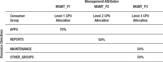
Figure 7-18. IORM intradatabase plan

Figure 7-19 shows the actual ratio of I/O requests scheduled for our IORM consumer groups during our stress test. A quick glance at the pie chart tells us that our IORM plan was definitely managing I/O resources at the consumer group level. You can see that the APPS consumer group does in fact take priority over all other groups. As expected, I/O is disproportionately allocated to the APPS group in the SCRATCH database (43.87%) compared to the APPS group in the SNIFF database (19.13%). This is because of the influence our Interdatabase Resource Plan has over our Intradatabase Resource Plan. Recall that our Interdatabase Plan grants a higher priority to the SCRATCH database (60% at level 1) than the SNIFF database (80% at level 2). The other IORM consumer groups follow a similar pattern.

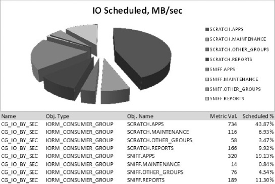
Figure 7-19. I/O operations scheduled per second, by consumer group

Other Processes Managed by IORM

There are a few internal processes managed by IORM that don't quite fit anywhere else in this chapter so we'll discuss them here. These internal processes are:

• Fast File Creation
• ETL (extract, transform, load)
• Recovery Manager

Exadata provides a feature called Fast File Creation for creating and extending database datafiles. It provides extremely fast I/O for creating and growing files in the storage grid. Generally speaking, this is a good thing. But how does Exadata manage the priority of certain, low priority, highly I/O intensive processes? The answer is IORM.

Fast File Creation

Exadata provides a feature called Fast File Creation, which brings all the I/O resources of the storage cells to bear in order to make quick work of creating and extending tablespace database files. But as you might imagine, if run unchecked, Fast File Creation can steal valuable resources from other database critical, and business critical processes. To prevent this, the FASTFILECRE function, which performs Fast File Creation, is mapped to a hidden IORM consumer group and assigned a priority below that of all other database foreground and background processes. When the storage cells are busy, Fast File Creation is throttled back so it doesn't degrade other processes. But when the storage cells are not busy, IORM allows it to consume all available I/O resources.

If you want to increase the priority of Fast File Creation, add a new consumer group mapping rule to switch it to another consumer group (with higher priority). The mapping rule must use the mapping attribute DBMS_RESOURCE_MANAGER.ORACLE_FUNCTION with a value set to the name of the Fast File Creation function, FASTFILECRE. For example, we can reassign the FASTFILECRE function to the MAINTENANCE consumer group we created earlier in the chapter as follows.

ETL

Depending on the database, extract, transform, and load (ETL) processes may be considered low-priority, or they may be absolutely-mission critical to the business. Oracle provides two built-in DBRM resource plans to manage the priority for typical ETL processes. The ETL_GROUP is set up with lower priority in the built-in DW_PLAN resource plan and, as the name implies, is given a much higher priority in the built-in ETL_CRITICAL_PLAN resource plan. Figures 7-20 and 7-21 show the default settings for these two resource plans.

Figure 7-20. DW_PLAN resource plan

Figure 7-21. ETL_CRITICAL_PLAN resource plan

Data Pump runs under the built-in DATALOAD function, which by default maps to the ETL_GROUP consumer group. Other programs, such as SQL Loader, may also be mapped to the ETL_GROUP using mapping rules we discussed earlier in the chapter. For example, the SQL Loader command is mapped to the ETL_GROUP consumer group as follows:

Recovery Manager

Exadata requires ASM for a database to access the storage grid. As such, Recovery Manager (Rman) is the required tool for executing database backup and recovery. Backups are a very I/O-intensive operation. For a number of years now, Rman has provided two ways to manage the load backups put on the I/O subsystem: backup channels and rate. The number of backup channels can be used to increase or decrease performance and load. Finer-grained control is provided through the rate parameter, which controls the rate in bytes per second that Rman streams to the backup channels. Exadata provides IORM management for Rman by mapping backup operations to the BACKUP function and copy operations to the COPY function. By default, the BACKUP, and COPY functions map to the built-in BATCH_GROUP consumer group. Similar to the FASTFILECRE function we described for Fast File Creation, the BACKUP and COPY functions may be mapped to any other consumer group in order to adjust their IORM priorities. For example, we can remap the BACKUP function to our MAINTENANCE consumer group as follows:

Summary

One of the biggest challenges for DBAs is effectively managing system resources to meet business objectives. Over the years Oracle has developed a rich set of features that make resource management a reality. Unfortunately, these features are rarely implemented due to their complexity. But make no mistake, as servers become more powerful and efficient, database consolidation is going to become increasingly common. This is especially true of the Exadata platform. Understanding how to leverage database and I/O resource management is going to become an increasingly important tool for ensuring that your databases meet the demands of your business. The best advice we can offer is to keep things simple. Attempting to make use of every bell and whistle in Oracle Resource Manager can lead to confusion and undesirable results. If you do not have a specific need for multi-level resource plans, then stick to the single-level approach; they are easy to implement and measure, and they work great in most situations. Category plans are another rarely needed feature. A majority of the situations you will face can be resolved by implementing a simple, single-level Interdatabase Resource Plan. So again, start small, keep it simple, and add features as you need them.