
Chapter 7. Analyzing Risk with Code Complexity
My uncle Frank has fished the rivers of Montana his entire life. To this day, he is a great fisherman. He always knows which combinations of pole, line, and bait have the best chance of catching a fish, and his friends consider him an expert in the field. As good as he is at fishing, he can’t catch fish if there aren’t any in the area of the river where he is fishing. He knows that great equipment and bait aren’t enough, so he also knows how to read depth and flow of the rivers and uses this information to predict accurately where fish will be. The combination of knowing what to do and developing a strategy based on analysis of the fishing area is what makes him so successful.
Techniques such as boundary-value analysis and pairwise testing are effective for reducing the number of needed test cases while minimally affecting risk. The problem is that there is not an even distribution of bugs throughout the source code. In fact, in a typical software project, some components tend to have many bugs while others have few or none. My uncle uses a variety of techniques to predict where the fish will be. Similarly, one of the necessities of software testing is to anticipate where pockets of bugs will be, and then target test cases toward those areas of the project.
Risky Business
Testing is often a process of managing risk. Risk-based testing is an approach to testing based on mitigating potential risks in a product. This approach intends to focus available testing resources on the most appropriate areas. In a sense, all testing is risk based; it is not possible to test everything, so as testers, we make choices based on a variety of criteria on where to concentrate our testing efforts.
Italian economist Vilfredo Pareto created a formula to describe the irregular distribution of wealth in his country, observing that 80 percent of the wealth belonged to 20 percent of the people. Many people believe that the Pareto principle[1]. (the 80:20 rule) applies as well to software projects. Applied generally, the Pareto principle states that in many measurements, 80 percent of the results come from 20 percent of the causes. When applied to software, the Pareto principle can mean that 80 percent of the users will use 20 percent of the functionality, that 80 percent of the bugs will be in 20 percent of the product, or that 80 percent of the execution time occurs in 20 percent of the code. One aspect of a risk-based approach attempts to classify which portion of the product contains these popular user scenarios and drives the creation of more tests directed at that portion of the product. The other side of the risk in this approach is that this approach relies on accurately determining where the majority of the testing effort should be and misses the fact that there will be customers who will use the features and code paths that fall outside of the 20 percent range.
Another manner in which to apply risk-based testing is to write more tests for the parts of the product that have a higher potential of containing bugs. Just as my uncle knows where to cast his line to have the best chance of catching a fish, a risk-based testing approach knows which tests to run to have the best chance of finding critical bugs.
A Complex Problem
Complexity is everywhere. I remember making chocolate chip cookies ever since I was old enough to reach the knobs on the oven. I used my grandmother’s recipe, and it only included a few ingredients. I rarely referred to the recipe, but the cookies were perfect every time. The measurements of the various ingredients were consistent (that is, two sticks of butter, two cups of flour, one cup each of white and brown sugar, and one bag of chocolate chips), and the cooking time was a round number (10 minutes). The key to my success was that the recipe was simple. Barring a catastrophe (such as rancid butter or a broken oven), I could not find a way to make bad chocolate chip cookies.
As an adult, I still love to cook, but I have run into various problems many times in the kitchen while attempting to reproduce a favorite dish or re-create a recipe inspired by the pictures included in some of my cookbooks. Recipes with dozens of ingredients and multiple cooking steps are primed for mistakes to happen. Usually, I make it through unscathed, but often enough, I end up with three pans cooking on the stove before I realize that I missed an entire step or misread the recipe and put a tablespoon of cayenne pepper into the soup instead of a teaspoon. The complexity of the recipe and the interaction of dealing with multiple recipes at once make it more likely that I will make a mistake. Similarly, complex code and interactions of complex portions of code are generally more prone to mistakes.
One method sometimes used to predict where bugs might be is to seek out the areas where the code is more complicated. Complex code has a tendency to have more bugs, and simple code tends to have fewer bugs. Complicated code also has the enormous drawback of being much more difficult to maintain. Code complexity is an important measure of the “difficulty” of the code. The greater the complexity of the code, the more difficult the code is to test.
Gut feel or subjective measurement from cursory code review is at times sufficient for gauging code complexity. Code smell is a term used often in Agile programming circles that describes code that might be too complex because of large functions or a large number of dependencies. Smells are typically a subjective measurement that can depend on the programming language or environment, and they are useful for identifying code that potentially should be refactored or rewritten.
Any time simplicity isn’t part of the initial design and implementation of the software, there is potential for the code to grow into a nonmaintainable mess. Subjective methods such as intuition or gut feel can be effective means to identify complex code, but there are objective measures of code complexity that can assist in determining where bugs can be hiding.
The simplest measure of code complexity might be lines of code (LOC). An application with 1,000 lines of code typically is less complex than an application with 10,000 lines of code is. Mathematics alone can lead you to believe that the 10,000-line project would have 10 times as many bugs as the 1,000-line project, but in practice, the 10,000-line project often has many, many more bugs. However, because of discrepancies in how lines of code are counted (see the following section), as well as numerous other external factors, lines of source code is generally discarded as an accurate complexity metric. Many other complexity measurements can be used to predict where bugs can occur, and some of those measurements are described in subsequent sections.
Counting Lines of Code
How many lines of code are in a program? How can such a simple question be so difficult to answer? Let’s start with something simple:
if (x < 0)
    i = 1;
else
    i = 2;
The preceding excerpt contains four lines. How many does it contain if formatted like this?
if (x < 0) i = 1;
else i = 2;
You would have a hard time counting the second example as four lines—it is two lines, or at least it is formatted as two lines. Personally, I don’t like the formatting of either example. Given the same code, I’d prefer to write it like this:
if (x < 0)
{
    i = 1;
}
else
{
    i = 2;
}
So, is this example two, four, or eight lines long? The answer depends on whom you ask. Some LOC measurements count only statements (in C, for example, this includes only lines ending in a semicolon). Other measurements count all lines except blank lines and comments. Others still count the number of assembly instructions generated (each of the preceding examples generates the exact same assembly language or intermediate language when compiled as managed code).
Although there are many methods for counting LOC, all you have to do if you want to measure LOC is pick a method that you like, and use it consistently. Measuring program length through lines of code is rarely an actionable metric but is simple to calculate and has potential for such tasks as comparing the deltas between two versions of a product or two components in a project.
Measuring Cyclomatic Complexity
Computer programs contain thousands of decisions: If this happens, do that...unless the other thing happened, then do this first. Programs that contain numerous choices or decisions have more potential to contain failures and are often more difficult to test. One of the most common methods of determining the number of decisions in a program is by using a measurement called cyclomatic complexity. Cyclomatic complexity is a measurement developed by Thomas McCabe[2] that identifies the number of linearly independent paths (or decisions) in a function. A function that contains no conditional operators (such as conditional statements, loops, or ternary operators) has only one linearly independent path through the program. Conditional statements add branches to the program flow and create additional paths through the function.
Program maintenance becomes an issue when cyclomatic complexity numbers rise. Psychologists have demonstrated that the average person can hold only five to nine pieces of information in short-term memory at one time; thus, when the number of interrelated choices grows beyond five to nine there is a much higher potential for the programmer to make a mistake when modifying the code. Exceptionally high numbers of decisions can lead to code that is difficult to maintain and even more difficult to test.
The most common method of computing McCabe’s complexity measurement is by first creating a control flow graph based on the source code, and then calculating a result based on the graph. For example, consider the code in Example 7-1.
int CycloSampleOne(int input)
{
    int result;
    if (a < 10)
        result = 1;
    else
        result = 2;

    return result;
}
This code is represented by the control flow graph shown in Figure 7-1.
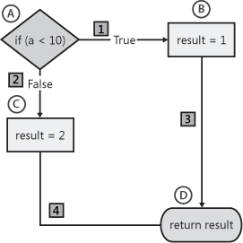
Based on the control flow graph, McCabe identifies the formula to calculate cyclomatic complexity for a function as edges – nodes + 2. In the graph in Figure 7-1, nodes appear as shapes, and the edges are the lines connecting the nodes that show potential paths through the program. The nodes in Figure 7-1 labeled A through D show the statements in the function. Using the formula described earlier, there are four nodes, and four edges, or paths between nodes. Analysis shows that the complexity of this function is 2 (edges (4) – nodes (4) + 2 = 2). An accurate shortcut to calculate cyclomatic complexity is simply to count the number of conditional (predicate) statements and add 1. In the preceding example, there is one condition (if (a < 10)), and thus the cyclomatic complexity is 2.
The code sample in Example 7-2 shows a slightly more complex (yet still relatively simple) example. The control flow graph in Figure 7-2 represents this code.
void CycloSampleTwo(int value)
{
    if (value !=0)
    {
        if (value < 0)
            value += 1;
        else
        {
           if (value == 999) //special value
               value = 0;
        else //process all other positive numbers
             value -= 1;
        }
    }
}
The previous two examples are in all probability much simpler than most code you will find in production, and creating a complete set of test cases for these code examples would be relatively quick work. For simple functions, calculation of cyclomatic complexity is straightforward and easily performed manually. For large functions with many decision points, or for automatically calculating cyclomatic complexity across a large code base, many tools are available (including tools from McCabe such as McCabe IQ,[3] or free tools such as CCCC, NDepend, and Code Analyzer). For managed code development, several free tools are on the market that calculate the cyclomatic complexity of a given piece of code, including Sourcemonitor, Reflector, and FxCop.
A primary use of cyclomatic complexity is as a measurement of the testability of a function. Table 7-1 contains McCabe’s guidelines on using cyclomatic complexity.
Cyclomatic complexity | Associated risk |
1–10 | Simple program with little risk |
11–20 | Moderate complexity and risk |
21–50 | High complexity and risk |
50+ | Very high risk/untestable |
Consider these values as guidelines. I have seen code with low cyclomatic complexity filled with bugs and code with cyclomatic complexity well over 50 that were well tested and contained few defects.
Halstead Metrics
Halstead metrics are an entirely different complexity metric based on the following four measurements of syntax elements in a program:
Number of unique operators (n1)
Number of unique operands (n2)
Total occurrences of operators (N1)
Total occurrences of operands (N2)
These measurements are used to derive a set of complexity metrics. For example, a measure of code length is determined by adding N1 and N2. Halstead metrics also can calculate a Difficulty metric with the following formula: (n1 / 2) * (N2 / n2). In the following code sample, there are six unique operators and four unique operands, used a total of 6 and 12 times each, respectively. Table 7-2 shows how I calculated these counts.
void HalsteadSample(int value)
{
    if (value !=0)
    {
        if (value < 0)
            value += 1;
        else
        {
           if (value == 999) //special value
               value = 0;

           else //process all other positive numbers
              value -= 1;
        }
    }
} |
n1 = 6
n2 = 4
N1 = 8
N2 = 12
Using Halstead metrics, the Length of this function is 18 (N1 + N2), and the Difficulty ((n1 / 2) * (N2 / n2)) is 9 ((6 / 2) * (12 / 4)).
Like cyclomatic complexity, Halstead metrics are valuable for determining the maintainability of a program, but there are varying views on this value ranging from “unreliable”[4] to “among the strongest measures of maintainability.”[5] As with cyclomatic complexity (and nearly every other metric I can think of), use this measurement primarily as an indicator of which code might need additional rework or analysis.
Object-Oriented Metrics
Object-oriented metrics are metrics related to classes and class structure in languages such as C++, Java, and C#. The most popular of these are the object-oriented metrics created by Chidamber and Kemerer[6] known as CK metrics. CK metrics include the following:
Advocates of object-oriented metrics suggest that classes with a large number of methods, deep inheritance trees, or excessive coupling are more difficult to test and maintain, and are more prone to contain defects.
In object-oriented programming, fan-in and fan-out metrics are a measurement of how many classes call into a specific class and how many classes are called from a specific class. For example, if a class contains methods called by 5 other classes and in turn calls methods in 10 other classes, its fan-in measurement is 5, and its fan-out measurement is 10. These measurements are frequently quite effective as maintainability metrics, but they also indicate where additional testing might be needed. For example, if a class is called by dozens of other classes (high fan-in measurement), there is a high potential for any code changes in that class to cause a new failure to occur in one of the calling classes.
Fan-in and fan-out measurements are also quite valuable in non-object-oriented programming when used at either the function or module level. Functions called by a high number of other functions can be some of the most difficult functions to maintain and test, and often simply cannot be changed. The biggest example of this I have seen in my career has been with Windows application programming interface (API) functions. Many of the core Windows functions are called by thousands of applications. Even the most trivial change to any of these functions has the potential to cause one of the calling functions to suddenly fail. Great care must be taken during maintenance of any function or module with a high fan-in measurement. From the testing perspective, this is a great place to be proactive. Determine as early as possible which functions, modules, or classes of your application will have the highest fan-in measurement, and concentrate testing efforts in that area.
Conversely, fan-out measurements tell you how many dependencies you have. If you have a function or class that calls 10 or 20 methods, this means there are 10 or 20 different methods where changes might affect you. This problem is often magnified when other developers or other teams entirely are responsible for the maintenance of these called functions.
High Cyclomatic Complexity Doesn’t Necessarily Mean “Buggy”
Being able to quantify how complex a given piece of software is doesn’t necessarily dictate an action item for the test team. It is possible for each of the preceding metrics to indicate a high level of complexity in code that contains very few bugs. I often refer to metrics such as this as smoke alarm metrics. When a smoke alarm starts screeching, it doesn’t guarantee that there is a fire, but it does indicate that you should look for a fire and respond appropriately. Similarly, when complexity metrics are high, it doesn’t necessarily mean that the code is “buggy” or unmaintainable; but it does mean that you should take a closer look.
For example, consider cyclomatic complexity and code using a long switch statement, such as the message loop used often in Windows programming. Each case statement in the loop creates a separate path and increases the cyclomatic complexity (and number of test cases needed) by one but doesn’t necessarily make the application difficult to test. Consider Microsoft Paint. Paint is quite simple compared to other graphic manipulation applications, but it has nearly 40 menu choices, another 16 choices for drawing tools, and another 28 choices for color selection. I didn’t look at the source code for Paint, but I wouldn’t be surprised if the code to handle all of these choices is contained in a single case statement! Add to this the drawing- and size-related messages that applications have to handle, and you have a function that some complexity metrics will tell you is so untestable that you should run screaming (but you probably shouldn’t).
The following code represents part of a typical Windows message loop. Message loops, by design, have dozens or more case statements resulting in a high measurement of cyclomatic complexity. Bugs in message loops definitely do occur, but not nearly in the amount that complexity metrics could lead you to believe.
int HandleMessage(message)
{
    switch (message)
    {
        case Move :
             // code omitted...
             break;


        case Size :
             // code omitted...
             break;


        ...
        // dozens more deleted
    }
}
In many other situations, however, you will likely find that areas of the source code with high complexity are also the areas that contain more bugs. Numerous studies have shown a high correlation between complexity metrics and bugs. Often, complexity is also associated with the maintainability of source code. Overly complex code is extremely difficult for maintenance programmers to work with. Getting familiar with the code requires extra time, and bug fixes or additional features can be challenging to implement without adding even more complexity to the code.
What to Do with Complexity Metrics
There are several other methods of measuring code complexity. Just about any reasonably well known complexity measurement likely has some merit and has demonstrated some success in identifying areas of code that might contain more bugs or be more difficult to maintain. Complexity measurements are all also quite capable of reporting false positives—that is, code that shows high complexity through analysis, but that contains few or no bugs and is simple to maintain. One method for moderating the false positives is to look at several different complexity metrics and combine, merge, or weigh the data to weed out some of the false positives. If several different complexity metrics all classify a function, module, or file as being highly complex, chances are that it actually might be more prone to containing bugs and could be difficult to maintain. On the other hand, if one measurement shows high complexity for a section of code, but other complexity measurements disagree, there is a realistic chance that the code is not too complex, too difficult to maintain, or prone to containing bugs.
What do you do with complex code? If it’s new code, high complexity indicates code that can need refactoring. Some teams at Microsoft have experimented with setting limits on the level of cyclomatic complexity for new functionality. (Most teams that have tried this have discovered that, by itself, cyclomatic complexity isn’t always an accurate indicator of code that is in need of refactoring.) Other teams, including the Windows team, look at a combination of several different complexity metrics and use the combined data to help determine the risk of changing a component late in the product cycle.
Consider, for example, the functions listed in Table 7-3. The OpenAccount function has high cyclomatic complexity but has few calling functions (fan in) and a low number of lines of code. This function might need additional rework to reduce the cyclomatic complexity, or review might show that the code is maintainable and that tests for all branches are easy to create. CloseAccount has a high number of calling functions but few branches. Additional inspection of this function might be warranted to reduce the number of calling functions, but this function probably does not have a significant amount of risk. Of the three functions, UpdatePassword might have the most risk. Cyclomatic complexity is moderate, there are nearly 20 calling functions, and the length of the function is nearly three times the length of the other functions. Of course, you want to test when changes are made to any of the functions, but the metrics for UpdatePassword should make you wary of any changes made at all to that function.
Function name | Cyclomatic complexity | Number of calling functions | Lines of code |
OpenAccount | 21 | 3 | 42 |
CloseAccount | 9 | 24 | 35 |
UpdatePassword | 17 | 18 | 113 |
The latest version of the Microsoft Visual Studio toolset contains measurements for complexity metrics, including cyclomatic complexity; Halstead metrics, shown in Figure 7-3 as maintainability index; and lines of code.

Summary
Code complexity is an essential metric for identifying where bugs might exist in your application and is equally valuable in identifying code that can cause maintenance issues. If you are not measuring complexity in any part of your code, start by measuring it in your most critical functionality or features. Over time, you can expand the scope of your complexity measurements and begin to compare complexity between components or feature areas.
Complexity is also an easy metric to misuse, so it is critical that you use the metrics wisely and monitor the value to ensure that these metrics are discovering what you expect them to discover. Remember that high complexity tells you only that the code might be prone to having more bugs. You might need additional investigation to know for sure.
[1] Wikipedia, “Pareto Principle,” http://en.wikipedia.org/wiki/Pareto_principle
[2] Thomas McCabe, “A Complexity Measure,” IEEE Transactions on Software Engineering SE-2, no. 4 (December 1996):308–320.
[3] McCabe IQ, home page, http://www.mccabe.com/iq.htm.
[4] Capers Jones, “Software Metrics: Good, Bad, and Missing,” Computer 27, no. 9 (September 1994): 98–100.
[5] P. Oman, HP-MAS: A Tool for Software Maintainability, Software Engineering (#91-08-TR) (Moscow, ID: Test Laboratory, University of Idaho, 1991).
[6] S. R. Chidamber and C. F. Kemerer, “A Metrics Suite for Object Oriented Design,” IEEE Transactions in Software Engineering 20, no. 6 (1994): 476–493.