
CHAPTER 2
RANDOM VARIABLES AND THEIR DISTRIBUTIONS
In a random experiment, frequently there has been greater interest for certain numerical values that can be deduced from the results of the random experiment than the experiment itself. Suppose, for example, that a fair coin is tossed consecutively six times and that we want to know the number of heads obtained. In this case, the sample space is equal to:
![]()
If we define X := “number of heads obtained”, then we have that X is a mapping of Ω to {1,2, ··· ,6}. Suppose, for example, we have X((H, H, T, H, H, T)) = 4. The mapping X is an example of a random variable. That is, a random variable is a function defined on a sample space. We will explain this concept in this chapter.
2.1 DEFINITIONS AND PROPERTIES
Definition 2.1 (Random Variable) Let(Ω, ![]() , P) be a probability space. A (real) random variable is a mapping
, P) be a probability space. A (real) random variable is a mapping ![]() such that, for all A
such that, for all A ![]() B,
B, ![]() , where B is the Borel σ-algebra over
, where B is the Borel σ-algebra over ![]() .
.
Note 2.1 Let (Ω, ![]() , P) be an arbitrary probability space. Given that the σ-algebra of Borel
, P) be an arbitrary probability space. Given that the σ-algebra of Borel ![]() in
in ![]() is generated by the collection of all the intervals of the form (–∞, x] with
is generated by the collection of all the intervals of the form (–∞, x] with ![]() , it can be demonstrated that a function
, it can be demonstrated that a function ![]() is a random variable if and only if
is a random variable if and only if ![]() for all
for all ![]() .
.
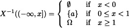
Let Ω = {a, b, c}, ![]() = {
= {![]() , {a}, {b, c}, Ω}, P be an arbitrary probability measure defined over
, {a}, {b, c}, Ω}, P be an arbitrary probability measure defined over ![]() . Assume
. Assume ![]() given by:
given by:
![]()
is a random variable since
while the mapping ![]() given by
given by
![]()
is not a random variable because:
![]()
If ![]() is taken as a σ-algebra over Ω, then Y is a random variable.
is taken as a σ-algebra over Ω, then Y is a random variable. ![]()
Consider the rolling of two dice. Ω = {(i,j), i, j = 1,2, ···, 6} is the set of all possible outcomes. Take ![]() = ℘(Ω). Let X defined by
= ℘(Ω). Let X defined by
![]()
be a random variable, due to ![]() for all
for all ![]() .
. ![]()
A light bulb is manufactured. It is then tested for its lifetime X by inserting it into a socket and the time elapsed (in hours) until it burns out is recorded. In this case, Ω = {t : t ≥ 0}. Take σ-algebra ![]() (see Example 1.11 and Exercise 9.1). Define:
(see Example 1.11 and Exercise 9.1). Define:
![]()
Then:
![]()
Hence, the lifetime X is a random variable. ![]()
Consider Example 2.3. Assume that the light bulbs so manufactured are being sold in the market and from past experience it is known that there will be a profit of $ 1.00 per bulb if the lifetime is less than 50 hours, a profit of $ 2.00 per bulb if the lifetime is between 50 and 150 hours and a profit of US$ 4.00 if the lifetime is more than 150 hours. Let Y be the profit function. Using the solution of Example 2.3, the profit function Y : X → ![]() is given by:
is given by:

Since Y satisfies ![]() for all
for all ![]() , Y is a random variable.
, Y is a random variable. ![]()
Let (Ω, ![]() , P) be a probability space and A
, P) be a probability space and A ![]()
![]() fixed. The function
fixed. The function ![]() given by
given by
![]()
is a real random variable. Indeed, if α ![]()
![]() , then:
, then:

The function χA is called an indicator function of A. Other notations frequently used for this function are IA and 1 A. ![]()
Notation 2.1 Let X be a random variable defined over the probability space (Ω, ![]() , P). It is also defined in the set notation form
, P). It is also defined in the set notation form
![]()
Theorem 2.1 Suppose that X is a random variable defined over the probability space (Ω, ![]() , P). The function PX defined over the σ-algebra
, P). The function PX defined over the σ-algebra ![]() through
through
![]()
is a probability measure over (![]() ,
, ![]() ) called the distribution of the random variable X.
) called the distribution of the random variable X.
Proof: It must be verified that PX satisfies the three conditions that define a probability measure:
- It is clear that, for all B

 , PX(B) ≥ 0.
 - PX(
 ) = P({ω Ω : X(ω) } = P(Ω) = 1.
 - Let A1, A2, ··· be elements of with
 for all i ≠ j. Then:

![]()
Let Ω = {a, b, c}, ![]() = {
= {![]() , {a}, {b, c}, Ω} and P be given by:
, {a}, {b, c}, Ω} and P be given by:

Let ![]() be given by:
be given by:
![]()
Then in this case we have, for example, that:

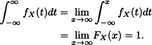
Definition 2.2 (Distribution Function) Let X be a real random variable. The function FX defined over ![]() through
through
![]()
is called the distribution function (or cumulative distribution function (cdf)) of the random variable X.
Consider Example 2.6. The distribution function of the random variable X is equal to:
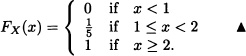
Let (Ω, ![]() , P) be a probability space and A
, P) be a probability space and A ![]()
![]() be fixed. The distribution function FX of the random variable χA is given by:
be fixed. The distribution function FX of the random variable χA is given by:

Consider the tossing of a fair coin three times and let X be a random variable defined by:
X := “number of heads obtained”.

Figure 2.1 Distribution function for Example 2.9
In this case, the distribution function of X is equal to
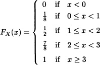
and its graph is shown in Figure 2.9. ![]()
Suppose a fair die is thrown two consecutive times. Let Z be a random variable given by:
Z := “absolute difference of the results obtained”.
That is:
Z((x, y)) = |x – y| with x, y ![]() {1, 2, 3, 4, 5, 6}.
{1, 2, 3, 4, 5, 6}.

Figure 2.2 Distribution function for Example 2.10
In this case the distribution function of the random variable Z is given by

and its graph is presented in Figure 2.10. ![]()
An important result of probability theory establishes that the distribution PX of a real random variable X is completely determined by its distribution function FX (see Muñoz and Blanco, 2002). The proof of this result is beyond the scope of the objectives of this book. Because of this, in the case of real random variables, it is common to identify the distribution of the variable as seen before as a probability measure over (![]() ,
, ![]() ) with its distribution function.
) with its distribution function.
It can be seen, in the previous examples, that the distribution functions of the random variables considered have certain common characteristics. For example, all of them are nondecreasing and right continuous and the limit when x tends to ∞ in all cases is 1; the limit when x tends to –∞ in all cases is equal to 0. These properties are characteristics of all distribution functions as it is stated in the next theorem.
Theorem 2.2 Let X be a real random variable defined over (Ω, ![]() , P). The distribution function FX satisfies the following conditions:
, P). The distribution function FX satisfies the following conditions:
1. If x < y, then FX(x) ≤ FX(y).
2. ![]()
3. ![]()
4. ![]()
Proof:
- If x < y, then:

- Let
 be fixed. Suppose that (xn)n is a decreasing sequence of real numbers with limit x. That is:

It can be seen that

and that

Therefore, from the probability measure P, it follows that:

- It is evident that for all n
 it is satisfied that

and


- It is clear that, for all n , it is satisfied that

and in addition that

Concluding:


It can be shown that any function F(x) satisfying conditions {1} – {4} of Theorem 2.2 is the distribution function of some random variable X.
Corollary 2.1 Let X be a real random variable defined over (Ω, ![]() , P), FX its distribution function and a,b
, P), FX its distribution function and a,b ![]()
![]() with a < b; then:
with a < b; then:

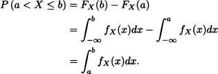
- P(a ≤ X ≤ b) = FX(b) – FX(a−).
- P(a < X ≤ b) = FX(b) – FX(a).
- P(a ≤ X < b) = FX(b−) – FX(a−).
- P(a < X < b) = FX(b−) – FX(a).
- P(X = a) = FX(a) – FX(a−).
- If P(a < X < b) = 0, then FX is constant in the interval (a, b).
Proof: Proof of the items 1 and 2 will be elaborated while the rest are left as exercises.
- Let be fixed. Suppose that (xn)n is an increasing sequence of real numbers with limit x. That is:

It is clear that

and


- Given:

It is obtained:

That is:

![]()
Which of the following functions can represent the cdf of a random variable X?
(a)

(b)

(c)

Solution: We will check all the four properties of F(x). For all three functions:
![]()
(a) The function F(x) is not a nondecreasing function.
(b) The function F(x) is not a nondecreasing function.
(c) The function F(x) satisfies all the four properties.
Hence, F(x) in (c) represents a cdf but F(x) in (a) and (b) does not. ![]()
The random variables are classified according to their distribution function. If the distribution function FX of the random variable X is a step function, then it is said that X is a discrete random variable. If FX is an absolutely continuous function, then it is said that X is a continuous random variable. And if FX can be expressed as a linear combination of a step function and a continuous function, then it is said that X is a mixed random variable.
Let X be a real random variable whose distribution function is given by:
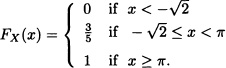
Then X is a discrete random variable. Notice that X takes only the values ![]() and π with probability
and π with probability ![]() and
and ![]() , respectively.
, respectively. ![]()
Let X be a random variable whose distribution function is given by

given that FX is a continuous function. Then X is a continuous random variable. ![]()
Let X be a random variable whose distribution function is given by
![]()
where 0 < q < 1. The distribution function has a jump at 0 since X takes the value 0 with probability q. Hence, X is a mixed random variable. ![]()
Note 2.2 If X is a real continuous random variable defined over the probability space (Ω, ![]() , P), then P(X = a) = 0 for all a
, P), then P(X = a) = 0 for all a ![]()
![]() .
.
2.2 DISCRETE RANDOM VARIABLES
The distribution of a discrete random variable has discontinuities that are called jumps. The corresponding points at which the jumps occur are called jump points. This concept will be established in a more precise way in the following definition.
Definition 2.3 Let X be a real random variable and FX its distribution function. It is said that FX presents a jump at the point a ![]()
![]() if:
if:
FX(a) − FX(a−) ≠ 0.
The difference FX(a−) – FX(a−) is called the magnitude of the jump or the jump value and by the properties developed previously it is equal to P(X = a).
In Example 2.10, it can be seen that the random variable Z has jump points z = i with i = 0,1, ··· , 5. The jump values are, ![]() and
and ![]() , respectively.
, respectively. ![]()
Note 2.3 If X is a real continuous random variable, then the collection of jump points of FX is an empty set.
The following result is very important since it guarantees that the number of jumps in a discrete real random variable is at most countable.
Theorem 2.3 Let X be a discrete real random variable defined over the probability space (Ω, ![]() , P) and FX its distribution function. Then the number of jumps of FX is at most countable.
, P) and FX its distribution function. Then the number of jumps of FX is at most countable.
Proof: (Hernandez, 2003) Given that the magnitude of each jump is an element belonging to the interval (0,1] and the collection of intervals In with the form
![]()
forms a partition of (0,1], it is obtained that the magnitude of each jump must belong to one of the intervals In. Because the magnitudes of the jumps are probabilities, it is clear that at most there is a jump whose magnitude is in the interval Io, there are at most three jumps whose magnitudes are in the interval I1, there are at most seven jumps with magnitudes in the interval I2 and in general, there are at most 2n+1 – 1 jumps whose magnitudes are in the interval In. Therefore, due to the existence of a countable number of intervals In and at most 2n+1 – 1 jumps in the interval In, it is concluded that the number of jumps is at most countable. ![]()
From the previous result it is concluded that the range of a discrete real random variable is at most a countable set.
Let X be a discrete real random variable and suppose that X takes the values x1, x2, ··· (all different). Let x be a real arbitrary number. Then:

That is, the distribution function of X is completely determined by the values of pi with i = 1,2, ··· where pi := P(X = xi). This observation motivates the following definition:
Definition 2.4 (Probability Mass Function) Let X be a discrete real random variable with values x1, x2, ··· (all different). The function pX defined in ![]() through
through
![]()
is called a probability mass function (pmf) of the discrete random variable X.
The following properties hold for the pmf:
- p(xi) ≥ 0 for all i and

Suppose that a fair die is tossed once and let X be a random variable that indicates the result obtained. In this case the possible values of X obtained are 1, ··· , 6. The probability mass function of X is given by:
![]()
It has been seen that the probability mass function of the discrete random variable X determines completely its distribution function. Conversely, it is obtained that for any x ![]()
![]() it is satisfied that:
it is satisfied that:
P(X = x) = FX(x) – FX(x−).
That is, the distribution function of the discrete random variable X determines completely its probability mass function.
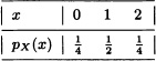
Let X be a random variable whose distribution function is given by:

In this case, the probability mass function of the random variable X is given by:

Let X be a discrete random variable with probability mass function given by:

In this case, the distribution function of the random variable X is given by:

Let X be a discrete random variable with values {0, ±1, ±2}. Suppose that P(X = –2) = P(X = –1) and P(X = 1) = P(X = 2) with the information that P(X > 0) = P(X < 0) = P(X = 0). Find the probability mass function and distribution function of the random variable X.
Solution: Let

Given:
P(X > 0) = P(X < 0) = P(X = 0).
Hence, 2α = 2β. Therefore:
P(X > 0) = 2α, P(X < 0) = 2α and P(X = 0) = 2α.
Assuming total probability is 1, ![]() . The probability mass function of the random variable X is given by:
. The probability mass function of the random variable X is given by:

The distribution function of the random variable X is given by:

A fair coin is tossed two times. Let X be the number of heads obtained.
- Find the probability mass function of the random variable X.
- Determine P(0.5 < X ≤ 4), P(–1.5 ≤ X ≤ 1) and P(X ≤ 2).
Solution:
- The random variable X takes values 0, 1 and 2:

The probability mass function of the random variable X is given by
-

A random variable X can take all nonnegative integer values and P(X = m) is proportional to αm(0 < α < 1). Find P(X = 1).
Solution: Let pm = P(X = m) = kαm where k is a constant. Also since pm is a pmf, we have:

2.3 CONTINUOUS RANDOM VARIABLES
In the study of continuous random variables, special emphasis is paid to the absolutely continuous random variables defined as follows:
Definition 2.5 (Absolute Continuous Random Variables)
Let X be a real random variable defined over the probability space (Ω, ![]() , P). It is said that X is absolutely continuous if and only if there exists a nonnegative and integrable real function fX such that for all x
, P). It is said that X is absolutely continuous if and only if there exists a nonnegative and integrable real function fX such that for all x ![]()
![]() it is satisfied that:
it is satisfied that:
The function fX receives the name probability density function (pdf) or simply density function of the continuous random variable X.
Note 2.4 A probability density function f satisfies the follomng properties:
(a) f(x) ≥ 0 for all possible values of x.
(b) ![]()
Property (a) follows from the fact that F(x) is nondecreasing and hence its derivative f(x) ≥ 0, while (b) follows from the condition that ![]() . It is clear that any real-valued function satisfying the above two properties will be a probability density function of some continuous random variable.
. It is clear that any real-valued function satisfying the above two properties will be a probability density function of some continuous random variable.
Let X be a random variable with distribution function given by:

The function fX defined by fx(x)
![]()
is a pdf of the random variable X. ![]()
Let X be a random variable with distribution function given by:

It is easy to verify that the function fX given by
![]()
is a pdf of the random variable X. ![]()
Suppose that X is an absolutely continuous random variable with probability density function fX. Some properties that satisfy this function will be deduced shortly.
It is known that:
If a, b ![]()
![]() , then:
, then:
Notice that because FX is a continuous function, the previous integral is also equal to P(a ≤ X ≤ 6), P(a ≤ X ≤ b) and P(a ≤ X < b). Moreover, it is obtained that
for all Borel sets B. The proof of this result is beyond the scope of this text. It is clear that the integral given in (2.2) must be interpreted as a Lebesgue integral given that the Riemannn integral is not defined for all Boolean sets. Nevertheless, if B is an interval or a union of intervals, it makes sense that, for practical effects, the Riemann integral is sufficient.
Since FX(x) is absolutely continuous, it is differentiable at all x except perhaps at a countable number of points. Using the fundamental theorem of integrals, we have ![]() for all x where FX(x) is differentiable. For the points a1, a2, ··· , an, ···, where FX(x) is not differentiable, we define:
for all x where FX(x) is differentiable. For the points a1, a2, ··· , an, ···, where FX(x) is not differentiable, we define:
![]()
With this we can conclude that:
![]()
This last property implies that, for Δx ≈ 0, it is obtained that:
![]()
That is, the probability that X belongs to an interval of small length around x is the same as the probability density function of X evaluated in x times the interval’s length.
When the context in which the random variable is referenced is clear, we will eliminate the subscript X in the distribution function as well as in the density function.
Let X be a random variable with density function given by:
![]()
Determine:
- The value of k.
- The distribution function of the random variable X.
- P(−1 ≤ X ≤
 ).
).
Solution:
- Given that

It is obtained that k = 6.
-

-

Consider Example 2.3. Let X be the random variable representing the lifetime of the light bulb. The cdf of X is given by:

- Determine k.
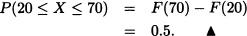
- Find the probability that the light bulb lasts more than 20 hours but no more than 70 hours.
Solution:
- Since F(x) is a cumulative distribution function of the continuous random variable X, it is a continuous function. Applying right continuity at x = 100, we get:

- The probability that the light bulb lasts more than 20 hours but no more than 70 hours is given by:
Let X be a random variable whose distribution function is given by:
![]()
Solution:

A continuous random variable X has density function given by
![]()
where λ > 0.
- Determine k.
- Find the distribution function of X.
Solution:
- Given that

It is obtained that k = λ2.
-

2.4 DISTRIBUTION OF A FUNCTION OF A RANDOM VARIABLE
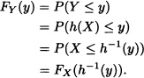
Suppose that X is a real random variable defined over the probability space (Ω, ![]() , P) and let g be a function such that Y = g(X) is a random variable defined over (Ω,
, P) and let g be a function such that Y = g(X) is a random variable defined over (Ω, ![]() , P). We are interested in determining (if possible) the distribution function of the random variable Y in terms of the distribution function of the random variable X.
, P). We are interested in determining (if possible) the distribution function of the random variable Y in terms of the distribution function of the random variable X.
Let X be a random variable and Y be defined as Y =| X |. We know that the modulus function is continuous and hence Y is also a random variable. Let FX be the cdf of X. The cdf of Y is given by:

If X is a continuous random variable, then P(X = –y) = 0. When X is a continous random variable, the cdf of Y is given by:
![]()
When X is a discrete random variable, the cdf of Y is given by:
![]()
Let X be a random variable with cdf ![]() . Find the cdf of Y = X+.
. Find the cdf of Y = X+.
Solution: We know that:
![]()

The distribution function of Y has a jump at 0. Hence, Y is a mixed random variable. ![]()
Let X be a discrete or continuous real random variable. Find the cdf of Y := aX + b where a, b ![]()
![]() and a ≠ 0.
and a ≠ 0.
Solution: It is clear that:

Let X be a real random variable with density function given by:
![]()

Therefore, the density function of the random variable Y is given by:

Let X be a real random variable with density function given by:
![]()
Let Y = eX. In this case, it is obtained that:

Therefore, the density function of the random variable Y is given by:

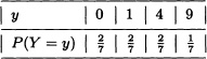
The distribution of a random variable X is given by:

Find the distribution of Y = αX + β, α > 0.
Solution: Since the distribution function of X has jumps at 0 and 1, X is a mixed random variable. Using Y = αX + β, the distribution function of Y is given by:

Note that the distribution function of Y has jumps at β and α + β. Hence, Y is also a mixed random variable. ![]()
Let X be a discrete random variable with probability mass function given by:

Let Y = X2. It can be seen that the possible values of Y are 0,1,4 and 9. Additionally:
The corresponding distribution functions of X and of Y are:

Let X be a random variable with probability mass function ![]() . Find the distribution of Y = n – X.
. Find the distribution of Y = n – X.
Solution: The pmf of Y is given by:

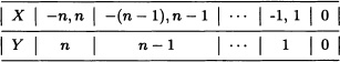
Let X be a random variable with distribution over the set of integers {–n, –(n – 1),··· , –1, 0, 1, ··· , (n – 1), n} given by:
![]()
Find the distribution of (i) | X | and (ii) X2.
Solution: (i) Let Y =| X |. For values of X, the corresponding values of Y are given in the following table:
For y = 0:
![]()
For y = 1,2, ··· , n:
![]()
Hence, the probability mass function of Y is given by:

(ii) Let Y = X2. Using a similar approach, the probability mass function of Y is given by

Suppose that X is a continuous random variable. Define:
![]()
Find the cdf of Y.
Solution:
![]()
Therefore:

In this example, note that X is a continuous random variable while Y is a discrete random variable. ![]()
Theorem 2.4 Let X be an absolutely continuous real random variable with density function fX. If h is a strictly monotonous and differentiable function, then the probability density function of the random variable Y = h(X) is given by
![]()
where h−1(·) is the unique inverse function of h(·).
Proof: Suppose that h is a strictly increasing function and let y ![]()
![]() such that y = h(x) for some x.
such that y = h(x) for some x.
Then:
Differentiating yields
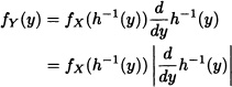
given that the derivative of h is positive.
Let h be a strictly decreasing function and y ![]()
![]() such that y = h(x) for some x. Then:
such that y = h(x) for some x. Then:

Differentiating yields

because in this case the derivative of h is negative.
If y ![]()
![]() is such that y ≠ h(x) for all x, then, FY(y) = 0 or FY (y) = 1, that is, fY(y) = 0.
is such that y ≠ h(x) for all x, then, FY(y) = 0 or FY (y) = 1, that is, fY(y) = 0.
Corollary 2.2 Let h be piecewise strictly monotone and continuously differentiable, that is, there exist intervals I1, I2, ··· , In which partition ![]() such that h is strictly monotone and continuously differentiable on the interior of each Ii. Let Y = h(X). Then the density of Y exists and is given by
such that h is strictly monotone and continuously differentiable on the interior of each Ii. Let Y = h(X). Then the density of Y exists and is given by
![]()
where hk−1 is the inverse of h in Ik.
Let X denote the measurement error in a certain physical experiment and let Y denote the square of the defined random variable X. Given that the pdf of X is known, find the pdf of Y.
Solution: Given that X is a continuous random variable and it denotes the error in the physical experiment. In order to find the pdf of the newly defined random variable Y, we shall first obtain the cdf of Y and then by differentiating the cdf we will obtain the corresponding pdf.
Let FX(x) denote the cdf of the given random variable X. The cdf of Y is given by:

Thus, we have obtained the cdf of the newly defined random variable Y. Now, by differentiating the cdf of Y, we get the pdf of Y:
![]()
Let X be a random variable with distribution
![]()
Define Y = eX. Find the pdf of Y.
Solution: Consider Y = h(X) = eX is a strictly increasing function of x and also h(X) is differentiable. Now:
y = h(x) = ex.
Then:

Since Y = eX satisfies all the conditions of Theorem 2.4, we get:
![]()
Hence, the pdf of Y is given by:

2.5 EXPECTED VALUE AND VARIANCE OF A RANDOM VARIABLE
Let X be a real random variable. It is known that its probabilistic-type properties are determined by its distribution function FX(·). Nevertheless, it is important to know a group of values that “summarize” in a certain way this information. For example, we want to define an “average” of the values taken by X and a measurement that “quantifies” by how much the values of X vary with respect to that value. This information will be given by two real values called expected value (average) and variance of the random variable, respectively. These concepts are stated precisely in the next definitions.
Definition 2.6 (Expected Value) Let X be a real random variable defined over the probability space (Ω, ![]() , P).
, P).
1. If X is a discrete random variable with values x1, x2, ···, it is said that X has an expected value if:
![]()
In such a way, the expected value E(X) (mathematical expectation, average) of X is determined as:
![]()
2. If X is a continuous random variable with density function fX, it is said that X has an expected value if:
![]()
In this case, the expected value E(X) (mathematical expectation, average) of X is determined as:
![]()
Note 2.5 If X is a real random variable that takes only a finite number of values, then E(X) always exists.
![]() EXAMPLE 2.40
EXAMPLE 2.40
Suppose that a normal die is thrown once and let X be a random variable that represents the result obtained. It is clear that:
![]()
Let (Ω, ![]() , P) be an arbitrary probability space and A
, P) be an arbitrary probability space and A ![]()
![]() fixed. It is known that X := χA is a discrete random variable that only takes the values 0 and 1 with probability P(Ac) and P(A), respectively. Therefore, E(X) exists and it is equal to P(A).
fixed. It is known that X := χA is a discrete random variable that only takes the values 0 and 1 with probability P(Ac) and P(A), respectively. Therefore, E(X) exists and it is equal to P(A). ![]()
Let X be a discrete random variable with pmf given by:
![]()

Let X be a continuous random variable with pdf given by:
![]()
Given that:
![]()
It is concluded that the expected value of X exists and it is equal to ![]() .
. ![]()
Let X be a random variable with values in ![]() . Suppose that
. Suppose that
![]()
where c > 0 is a constant such that
![]()
Given that
![]()
E(X) does not exist. ![]()
Let X be an absolutely continuous random variable with density function given by
![]()
where α > 0 is a constant.
Then
![]()
which means that E(X) does not exist. ![]()
The following result allows us to find the expected value of an absolutely continuous random variable from its distribution function.
Theorem 2.5 Let Y be an absolutely continuous random variable with density function f. If E(Y) exists, then:
![]()
Proof:

This is illustrated in Figure 2.3. ![]()
Sometimes we are faced with a situation where we must deal not with the random variable whose distribution is known but rather with some function of the random variable as discussed in the previous section.
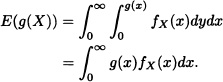
Suppose that X is a random variable. Let ![]() be a function such that Y = g(X) is also a random variable and whose expected value exists. It is clear that, to calculate E(Y), we need to find the density function of the random variable Y. However, fortunately there is a method that allows us to do the calculations in a simpler way, known as the “law of the unconscious statistician”. This method has been stated in the following theorem.
be a function such that Y = g(X) is also a random variable and whose expected value exists. It is clear that, to calculate E(Y), we need to find the density function of the random variable Y. However, fortunately there is a method that allows us to do the calculations in a simpler way, known as the “law of the unconscious statistician”. This method has been stated in the following theorem.

Figure 2.3 Illustration of expectation value for continuous random variable
Theorem 2.6 Let X be a real random variable with density function fX and ![]() a function such that Y = g(X) is a random variable. Then
a function such that Y = g(X) is a random variable. Then

whenever the sum, in the discrete case, or the integral in the continuous case converges absolutely.
Proof:
- Suppose that X is a discrete random variable that takes the values x1, x2, ···. In this case the probability mass function of X is given by:

The random variable Y = g(X) takes the values g(x1), g(x2), ···. It is clear that some of these values can be the same. Let us suppose that yj with j ≥ 1 represents different values of g(xi). Then, grouping all the
g(xi) that have the same value, it can be obtained that:

- Let X be an absolutely continuous random variable with density function fX. Suppose that g is a nonnegative function. Then

where B := {x: g(x) > y}. Therefore:
The proof for the general case requires results that are beyond the scope of this text. The interested reader may find them in the text of Ash (1972).
![]()
Let X be a continuous random variable with density function given by:
![]()

Next, some important properties of the expected value of a random variable are presented.
Theorem 2.7 Let X be a real random variable.
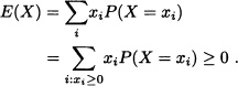
1. If P(X ≥ 0) = 1 and E(X) exists, then, E(X) ≥ 0.
2. E(α) = α for every constant α.
3. If X is bounded, that is, there exists a real constant M > 0 such that P(|X| ≤ M) = 1, then E(X) exists.
4. If α and β are constants and if g and h are functions such that g(X) and h(X) are random variables whose expected values exist, then the expected value of (αg(X) + βh(X)) exists and:
![]()
5. If g and h are functions such that g(X) and h(X) are random variables whose expected values exist and if g(x) ≤ h(x) for all x, then:
E(g(X)) ≤ E(h(X)).
In particular:
|E(X)| ≤ E(|X|).
Proof:
- Suppose that X is a discrete random variable that takes the values x1, x2, ···. Given that P(X < 0) = 0, it is obtained that P(X = xj) = 0 for all xj < 0. Therefore:
If X is an absolutely continuous random variable with density function f, then:

-

- If X is a discrete random variable that takes values x1, x2, ···, then, because P(|X| > M) = 0, it can be supposed that {x1, x2, ···}
 [–M, M]. In conclusion:
If X is an absolutely continuous random variable with density function f, then, given that P(|X| > M) = 0, it can be supposed that f(x) = 0 for all x
 [–M, M]. Therefore:
- The proof for the continuous case is elaborated here while the discrete case is left as an exercise. If X is an absolutely continuous random variable with density function f, then:

The expected value of (αg(X) + βh(X)) exists and it is clear that:

- The proof for the continuous case is elaborated here while the discrete case is left as an exercise. If X is an absolutely continuous random variable with density function f, then:

Given that
–|X|≤ X ≤ |X|
it is obtained that:
E(–|X|) ≤ E(X) ≤ E|X|
–E(|X|) ≤ E(X) ≤ E(|X|).That is:
|E(X)| ≤ E(|X|).
![]()
The expected value of the random variable is the “first central moment” of a variable around zero. In general, central moments around zero of random variables are the expected values of the power of the variable. More precisely:
Definition 2.7 (Central Moment Around Zero)
Let X be a real random variable. The rth central moment of X around zero, denoted by μ′r, is defined as
μ′r := E(Xr)
whenever the expected value exists.
The following result allows to confirm that if s < r and μ′r exists, then μ′s exists.
Theorem 2.8 If X is a random variable such that μ′r exists, then μ′s exists for all s < r.
Proof: Proof for the continuous case is elaborated here while the discrete case is left for the reader.
Given that
![]()

![]()
Definition 2.8 (Central Moment Around the Average) Let X be a real random variable whose expected value exists. The rth central moment of X around E(X) is defined as
μr := E([X – E(X)]r)
whenever the expected value exists.
The following result allows to relate the rth order moments around the mean with the rth order moments around the origin.
Theorem 2.9 Let X be a random variable whose expected value exists. If μr exists, then:
![]()
Proof:

![]()
Note that for any random variable whose expected value exists it is satisfied that μo = 1 and μ1 = 0. The second central moment of X, around the mean, receives the name of variance of the random variable X and it is generally denoted by σ2X ; the square root of the variance is called standard deviation of X and it is denoted usually by σX. Other notations with frequent use for the variance of X are Var(X) and V(X). In this text, any of these notations will be used indistinctively.
The variance measures the dispersion of the values of the variable around its mean. The term (X – E(X))2 is the square of the distance from X to E(X) and therefore, E(X – E(X))2 represents the average of the squares of the distances of each value from X to E(X). Then, if a random variable has a small variance, the possible values of X will be very close to the mean, while if X has large variance, then the values of X tend to be far away from the mean.
In the applications (see Ospina, 2001) a measure of relative dispersion is commonly used. It is called variation coefficient and is defined as:
![]()
When |E(X)| is not near zero, CV (X) is used as an indicator of how large the variance is. Empirically, it has been seen that when |CV (X)| < 0.1 the variance generally is small.
Some important properties of the variance of a random variable are presented next.
Theorem 2.10 Let X be a random variable whose expected value exists and α, β ![]()
![]() are constants. Then:
are constants. Then:
1. Var(X) ≥ 0.
2. Var(α) = 0.
3. Var(αX) = α2Var(X).
4. Var(X + β) = Var(X).
5. Var(X) = 0 if and only if P(X = E(X)) = 1.
Proof:
- It is clear from the definition of variance and from the properties of the expected value.
-
Var(α) = E(α – E(α))2 = E(0) = 0.
-

-

- (a) If X = E(X) with probability 1, it is clear that Var(X) = 0.
(b) Suppose that Var(X) = 0, and let a := E(X).
If P(X = a) < 1, then c > 0 exists such that
P((X – a)2 > c) > 0
given that

Then

which is a contradiction. Therefore P(X = E(X)) = 1.
![]()
To calculate the variance of a random variable, the following result will be very useful.
Theorem 2.11 Let X be a random variable whose E(X2) exists. Then:
Var(X) = E(X2) – (E(X))2.
Proof:

![]()
Suppose that a fair die is thrown once and let X be a random variable that represents the result obtained. It is known that ![]() and:
and:
![]()
Then:
![]()
Let X be defined as in Example 2.41. Then:
E(X2) = P(X = 1) = P(A).
Therefore:
![]()
Let X be defined as in Example 2.42. Then in this case:

Therefore:
![]()
Let X be defined as in Example 2.43. Then:

Therefore:
![]()
The probability generating function (pgf) plays an important role in many areas of applied probability, in particular, in stochastic processes. In this section we will discuss pgf’s, which are defined only for nonnegative integer valued random variables.
Definition 2.9 (Probability Generating Functions) Let X be a nonnegative integer-valued random variable and let pk = P(X = k), k = 0, 1, 2, ··· with ![]() . The pgf of X is defined as:
. The pgf of X is defined as:
![]()
Since GX(1) = 1, the series converges for |s| ≤ 1.
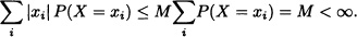
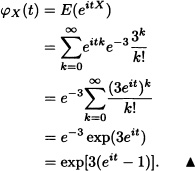
For λ > 0, let X be a discrete random variable with probability mass function given by:
![]()
Then:

Let X be a discrete random variable with probability mass function given by
![]()
where n is a positive integer and p ![]() (0, 1). Then:
(0, 1). Then:

Note 2.6 If X and Y have pgf’s GX(s) and GY(s), respectively, then GX(s) = GY(s) if and only if ![]()
Theorem 2.12 Let X be a nonnegative integer-valued random variable with E(|X|k) < ∞ for all k = 1,2, ···. Then, ![]() where
where ![]() is the rth derivative of its pgf GX(s) at s = 1.
is the rth derivative of its pgf GX(s) at s = 1.
Proof:
![]()
with pn = P(X = n), n = 0, 1, ···. Differentiate with respect to s, and it is assumed that the order of summation and differentiation can be interchanged. We have:
![]()
When s = 1:
![]()
In general:

Since the series is convergent for |s| ≤ 1 and using Abel’s lemma:
![]()
![]()
If GX(s) = eλ(s-1), |s| < 1, then:

The moments of a random variable X have a very important role in statistics not only for the theory but also for applied statistics. Due to this, it is very convenient to have mechanisms that allow easy calculations for the moments of the random variable. This mechanism is provided by the so-called moment generating function which will be as follows.
Definition 2.10 (Moment Generating Function) Let X be a random variable such that E(etX) is finite for all t ![]() (−α, α) with real positive α. The moment generating function (mgf) of X, denoted by mX(·), is defined as:
(−α, α) with real positive α. The moment generating function (mgf) of X, denoted by mX(·), is defined as:
mX(t) = E(etX) with t ![]() (–α, α).
(–α, α).
That is:

It is important to notice that not all probability distributions have moment generating functions associated with them. Later on some examples will be given that ratify this statement.
Before giving the important properties of the mgf of a random variable X, some examples are presented.
Let X be a discrete random variable with probability mass function given by
![]()
where n is a positive integer and p ![]() (0,1).
(0,1).
In this case:

Note 2.7 The distribution shown in Example 2.54 receives the name of binomial distribution with parameters n and p. In the next chapter, this distribution will be studied in detail.
Let X be the random variable as in Example 2.42. In this case:
Let X be a random variable with density function given by:
![]()

Let X be a random variable with density function given by

where μ ![]()
![]() and σ > 0 are constants.
and σ > 0 are constants.
Then:
![]()
With a change of variable
![]()
it is obtained that:

Given that ![]() it is deduced that for t > 0:
it is deduced that for t > 0:
![]()
Therefore, if ![]() is taken, it is obtained that
is taken, it is obtained that
![]()
Thus by taking
![]()
![]()
This means that there does not exist a neighborhood of the origin in which E(etX) is finite and in consequence the moment generating function of X does not exist. ![]()
The existence of the moment generating function of a random variable X guarantees the existence of all the rth order moments around zero of X. If the moment generating function exists, then it is differentiable in a neighborhood of the origin and satisfies
![]()
More precisely, the next two theorems state this and the proofs can be found in Hernandez (2003).
Theorem 2.13 If X is a random variable whose moment generating function exists, then E(Xr) exists for all r ![]() N.
N.
It is important to clarify that the converse of the previous theorem is not valid: the fact that all the rth order moments of a random variable X exist does not guarantee the existence of the mgf of the variable. For example, for the random variable in Example 2.57, it is known that for all r ![]()
![]() :
:
![]()
Theorem 2.14 If X is a random variable whose moment generating function mX(·) exists, then, h ![]() (0, ∞) exists such that:
(0, ∞) exists such that:
![]()
Therefore:
![]()
An important property of the mgf of a random variable is that, when it exists, it characterizes the distribution of the variable. More precisely, the following theorem is obtained. Its proof is beyond the scope of this text. The interested reader may refer to Ash (1972).
Theorem 2.15 Let X and Y be random variables whose moment generating functions exist. If
mX(t) = mY(t) for all t,
then X and Y have the same distribution.
As it can be seen, the moment generating function of a random variable, when it exists, is a very helpful tool to calculate the rth order moments around zero of a variable. Unfortunately, this function does not always exist, and thus it is necessary to introduce a new class of functions that are equally useful and always exist.
Definition 2.11 (Characteristic Function) Let X be a random variable. The characteristic function of X is the function ![]() defined by:
defined by:
![]()
Let X be a random variable with:
![]()
Then:

Let X be a discrete random variable with probability mass function given in Example 2.42. Then:
Let X be a continuous random variable with density function f given by:
![]()
Then, for t ≠ 0

and for t = 0
![]()
Next, some principal properties of the characteristic function, without proof, will be presented. The interested reader may consult these proofs in Grimmett and Stirzaker (2001) and Hernandez (2003).
Theorem 2.16 If X is a discrete or absolutely continuous random variable, then E(eitX) exists for all t ![]()
![]() .
.
Theorem 2.17 Let X be a random variable. The characteristic function φX(·) of X satisfies:
1. φX(0) = 1.
2. |φX(t) ≤ 1 for all t.
3. If E(Xk) exists, then:
![]()
Finally, it is important to notice that the characteristic function of a random variable, as in the case of mgf (when it exists), determines the distribution of the variable. That is, it satisfies:
Theorem 2.18 If X and Y are random variables and
![]()
then X and Y have the same distribution.
EXERCISES
2.1 Let Ω = {1,2,3}, ![]() = {
= {![]() , {1}, {2,3}, Ω}. Let us define, for A
, {1}, {2,3}, Ω}. Let us define, for A ![]()
![]() :
:
![]()
Is ![]() defined by X(ω) = ω2 a real random variable? Justify.
defined by X(ω) = ω2 a real random variable? Justify.
2.2 Let Ω = {1,2,3,4}. Determine the least σ-algebra over Ω so that X(ω) := ω + 1 is a real random variable.
2.3 A coin is biased in such a way that P(H) = ![]() and P(T) =
and P(T) = ![]() . Suppose that the coin is tossed three consecutive times and let X be the random variable that indicates the number of heads obtained. Find the distribution function of the random variable X and calculate E(X).
. Suppose that the coin is tossed three consecutive times and let X be the random variable that indicates the number of heads obtained. Find the distribution function of the random variable X and calculate E(X).
2.4 The sample space of a random experiment is Ω = {a, b, c, d, e, f} and each result is equally probable. Let us define the random variable X as follows:

Calculate the following probabilities:
a) P(X = 1).
b) P(|X – 1| ≤ 1).
c) P(X ≥ 0 or X < 2).
2.5 Prove that if all values of a real random variable X are in the interval [a, b] with a < b, then FX(x) = 0 for all x < a and FX(x) = 1 for all x ≥ b.
2.6 A fair coin is tossed four consecutive times. Let X be the random variable that denotes the number of heads obtained. Find the distribution function of the random variable Y := X – 2 and graph it.
2.7 Let (Ω, ![]() , P) be a probability space defined as follows:
, P) be a probability space defined as follows:
![]()
for all ω ![]() Ω. Consider the random variables Xn defined over Ω, as:
Ω. Consider the random variables Xn defined over Ω, as:
![]()
a) Determine the set of values S taken by the random variable Xn.
b) Verify that:
![]()
2.8 A box contains 5 white balls and 10 black ones. A die is thrown. A number of balls equal to the result obtained in the die are taken out of the box. What is the probability that all balls taken out of the box are white balls? What is the probability that the result obtained when throwing the die is 3 if all the balls taken out of the box are white?
2.9 Let X be a random variable with density function given by:

a) Determine the value of c.
b) Obtain the distribution function of the random variable X.
c) Calculate P(0 ≤ X < 0.5).
d) Determine P(X > 0.5 | X > 0.1).
e) Calculate the distribution function and the density function of the random variable Y := 2X + 3.
2.10 Let X be a random variable with density function given by:
![]()
a) Calculate the value of c.
b) Determine the distribution function of the random variable X.
c) Calculate P(|X| ≥ 0.2).
2.11 The cumulative distribution function of a random variable X is given by:

a) Calculate P(X ≥ ![]() ) and P(–2 ≤ X ≤
) and P(–2 ≤ X ≤ ![]() ).
).
b) Determine the density function fX (·) .
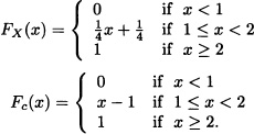
2.12 Let X, Y and Z be random variables whose distribution functions are respectively:
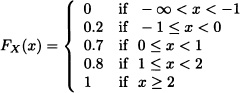

a) Which variables are discrete variables? Which variables are continuous variables? Explain.
b) Calculate P(X = 0), P(![]() < X ≤ 2) and P(X > 1.5).
< X ≤ 2) and P(X > 1.5).
c) Calculate P(Y = 0), P(![]() < Y ≤ 2) and P(Y > 0).
< Y ≤ 2) and P(Y > 0).
d) Calculate P(Z = 0), P(−![]() > Z ≤
> Z ≤ ![]() ) and P(Z ≥ 2).
) and P(Z ≥ 2).
2.13 A circular board with radius 1 is sectioned in n concentric discs with radii ![]() . A dart is thrown randomly inside the circle. If it hits the ring between the circles with radii
. A dart is thrown randomly inside the circle. If it hits the ring between the circles with radii ![]() and
and ![]() for i = 0, ··· , n – 1, n – i monetary units are won. Let X be the random variable that denotes the amount of money won. Find the probability mass function of the random variable X.
for i = 0, ··· , n – 1, n – i monetary units are won. Let X be the random variable that denotes the amount of money won. Find the probability mass function of the random variable X.
2.14 (Grimmett and Stirzaker, 2001) In each of the following exercises determine the value of the constant C so that the functions given are probability mass functions over the positive integers:
a) p(x) = C2−x .
b) ![]()
c) p(x) = Cx−2 .
d) ![]()
2.15 (Grimmett and Stirzaker, 2001) In each of the following exercises determine the value of the constant C so that the functions given are probability mass functions:
a) p(x) = C{x(1 – x)}−![]() , 0 < x < 1.
, 0 < x < 1.
b) p(x) = C exp(–x – e−x), x ![]()
![]() .
.
2.16 An absolutely continuous random variable X takes values in the interval [0,4] and its density function is given by:
![]()
b) Calculate P(![]() ≤ X < 3).
≤ X < 3).
2.17 Let X be an absolutely continuous random variable with density function f. Prove that the random variables X and –X have the same distribution function if and only if f(x) = f(–x) for all x ![]()
![]() .
.
2.18 In the following cases, determine the distribution function of the discrete random variable X whose probability mass function is given by:
a) P(X = k) = pqk–1, k = 1,2, ··· with p ![]() (0,1) fixed and q := 1 – p.
(0,1) fixed and q := 1 – p.
b)
![]()
2.19 A person asks for a key ring that has seven keys but he does not know which is the key that will open the lock. Therefore, he tries with each one of the keys until he opens the lock. Let X be the random variable that indicates the number of tries needed to achieve the goal of opening the lock.
a) Determine the density function of the random variable X.
b) Calculate P(X ≤ 2) and P(X = 5).
2.20 Four balls are taken out randomly and without replacement from each box that contains 25 balls numbered from 1 to 25. If you bet that at least 1 of the 4 balls taken out has a number less than or equal to 5, what is the probability that you win the bet?
2.21 A player takes out, simultaneously and randomly, 2 balls from a box that contains 8 white balls, 5 black balls and 3 blue balls. Suppose that the player wins 5000 pesos for each black ball selected and loses 3000 pesos for every white ball selected. Let X be the random variable that denotes the player’s fortune. Find the density function of the random variable X.
2.22 A salesman has two different stores where he sells computers. The probability that he sells, in one day, a computer in the first store is 0.4 and independently, the probability that he sells, in one day, a computer in the second store is 0.7. Additionally, suppose that it is equally probable that he sells a computer of type 1 or type 2. A type 1 computer costs $1800 while the type 2 computer, with the same specifications, costs $1000. Let X be the amount, in dollars, that the salesman sells in one day. Find the distribution of the random variable X.
2.23 Prove that
![]()
and use the above result to show that
![]()
is a density function if σ > 0.
2.24 Suppose that f and g are density functions and that 0 < λ < 1 is a constant. Is λf + (1 – λ)g a density function? Is fg a density function? Explain.
2.25 Let X be a random variable with cumulative distribution function given by:
Determine a cumulative discrete distribution function Fd(·) and one continuous Fc(·) and the constants α and β with α + β = 1 such that:
FX(x) = αFd(x) + βFc(x).
2.26 Let X be a random variable with cumulative distribution function given by:

Determine the cumulative discrete distribution function Fd(·) and one contin-uous Fc(·) and the constants α and β with α + β = 1 such that:
FX(x) = αFd(x) + βFc(x).
2.27 We say that a discrete real random variable X has Fisher logarithmic distribution with parameter θ if its density function is given by

with θ ![]() (0,1). Verify that p is a probability mass function.
(0,1). Verify that p is a probability mass function.
2.28 Let X be a random variable with distribution function given by:

Calculate Var(X).
2.29 Let X and Y be two nonnegative continuous random variables having respective cdf’s FX and FY. Suppose that for some constants a > 0 and b > 0:
![]()
Determine E(X) in terms of E(Y).
2.30 Let X be a continuous random variable with strictly increasing dis-tribution function F. What type of distribution have the random variable Y := –ln(FX(X))?
2.31 Let X be a random variable which can only take values –1,0,1 and 2 with P(X = 0) = 0.1, P(X = 1) = 0.4 and P(X = 2) = ![]() P (X = –1). Find E(X).
P (X = –1). Find E(X).
2.32 An exercise on a test for small children required to show the corre-spondence between each of three animal pictures with the word that identifies the animal. Let us define the random variable Y as the number of correct answers if a student assigns randomly the three words to the three pictures.
a) Find the probability distribution of Y.
b) Find E(Y) and Var(Y).
2.33 Let X be a random variable with density function given by:
![]()
a) Determine the value of C.
b) Calculate P(X ≥ 0).
c) Find (if they exist) E(X) and Var(X).
d) Find the distribution function of X.
2.34 A die is tossed two times. Let X and Y be the random variables defined by:
X := “result of the first throw”.
Y := “result of the second throw”.
Calculate E(max {X, Y}) and E(min {X, Y}).
2.35 Let X be a random variable with density function given by:

a) Calculate μ := E(X) and σ2 := Var(X).
b) Find P(μ – 2σ < X < μ + 2σ).
2.36 Let X be a random variable with density function given by:
![]()
a) Calculate μ := E(X) and σ2 := Var(X).
b) Determine the value of c so that ![]() .
.
2.37 Let X be a random variable with density function given by:
![]()
a) Determine the value of C.
b) Find (if they exist) the mean and variance of X.
2.38 Suppose that X is a continuous random variable with pdf fX(x) = e−x for x > 0. Find the pdf for the random variable Y given by:
![]()
2.39 Let X be a random variable with continuous and strictly increasing cumulative distribution function.
a) Determine the density function of the random variable Y := |X|.
b) Find the cumulative distribution function of the random variable Y := X3.
2.40 There are three boxes A, B and C. Box A contains 5 red balls and 4 white balls, box B contains 8 red balls and 5 white balls and box C contains 2 red balls and 6 white ones. A ball is taken out randomly from each box. Let X be the number of white balls taken out. Calculate the probability mass function of X.
2.41 Let X be a random variable with P(X = 0) = 0 and such that E(X) exits and is different from zero.
a) Is it valid to say, in general, that:
b) Is there a random variable X such that equation (2.3) is satisfied? Explain.
2.42 Let X be a discrete random variable with values in the nonnegative integers and such that E(X) and E(X2) exist.
a) Prove that:
![]()
b) Verify that:
![]()
2.43 Determine if the following propositions are true or false. Justify your answer.
a) If P(X > Y) = 1, then E(X) > E(Y).
b) If E(X) > E(Y), then P(X > Y) = 1.
c) If Y = X + 1, then FX (x) = FY (x + 1) for all x.
2.44 Let X be a random variable such that:
P(X = 1) = p = 1 – P(X = –1) .
Find a constant c ≠ 1 such that E (cX) = 1.
2.45 Let X be a random variable with values in ![]() + with
+ with ![]() .
.
a) Determine the value of C.
b) Find (if it exists) E(X).
2.46 Let X be a random variable with values ![]() , and such that
, and such that ![]() . Does E(X) exist? Does Var(X) exists? Explain.
. Does E(X) exist? Does Var(X) exists? Explain.
2.47 (Markov’s Inequality) Let X be a real random variable with X ≥ 0 and such that E(X) exists. Prove that, for all α > 0, it is satisfied that:
![]()
2.48 (Chebyschev’s Inequality) Let X be a random variable with mean μ and variance σ2.
a) Prove that for all ![]() > 0 it is satisfied that:
> 0 it is satisfied that:
![]()
b) If μ = σ2 = 20, what can be said about P (0 ≤ X ≤ 40)?
2.49 Let X be a random variable with mean 11 and variance 9. Use Chebyschev’s inequality to find (if possible):
a) A lower bound for P (6 < X < 16).
b) The value of k such that P(|X – 11| ≥ k) ≤ 0.09.
2.50 (Meyer, 1970) Let X be a random variable with mean μ and variance σ2. Suppose that H is a function two times differentiable in x = μ and that Y := H (X) is a random variable such that E(Y) and E(Y2) exist.
a) Prove the following approximations for E(Y) and Var (Y) :

b) Using the result in part (a), calculate (in an approximate way) the mean and variance of the random variable
Y := 2(1 – 0.005X)1.2
where X is a random variable whose density function is given by:
![]()
2.51 Find the characteristic function of the random variable X with probability function P(X = 1) = ![]() and P(X = 0) =
and P(X = 0) = ![]() .
.
2.52 Determine the characteristic function of the random variable X with density function given by
![]()
where a,b ![]()
![]() and a < b.
and a < b.
2.53 Determine the characteristic function of the random variable X with density function given by:
![]()
2.54 (Quartile of order q) For any random variable X, a quartile of order q with 0 < q < 1, is any number denoted by xq that satisfies simultaneously the conditions
(i) P(X ≤ xq) ≥ q
(ii) P(X ≥ xq) ≤ 1 – q .
The most frequent quartiles are x0.5, x0.25 and x0.75, named, respectively, median, lower quartile and upper quartile.
A quartile xq is not necessarily unique. When a quartile is not unique, there exists an interval in which every point satisfies the conditions (i) and (ii). In this case, some authors suggest to consider the lower value of the interval and others suggest the middle point of the interval (see Hernández, 2003). Taking into account this information, solve the following exercises:
a) Let X be a discrete random variable with density function given by:
![]()
Determine the lower quartile, the upper quartile and the median of X.
b) Let X be a random variable with density function given by:
![]()
Determine the mean and median of X.
c) Let X be a random variable with density function given by:
![]()
Determine (if they exist) the mean and the median of X.
2.55 (Mode) Let X be a random variable with density function f(.). A mode of X (if it exists) is a real number ζ such that:
![]()
a) Let X be a discrete random variable with density function given by

Find (if it exists) the mode of X.
b) Suppose that the random variable X with density function given by
![]()
where r > 0 and λ > 0 are constants and Γ is the function defined by:
![]()
If E(X) = 28 and the mode is 24, determine the values of r and λ.
c) Verify that if X is a random variable with density function given by
![]()
with a,b ![]()
![]() , a < b then any ζ
, a < b then any ζ ![]() (a, b) is a mode for X.
(a, b) is a mode for X.
d) Verify that if X is a random variable with density function given by
![]()
then the mode of X does not exist.
2.56 Suppose that the time (in minutes) that a phone call lasts is a random variable with density function given by:
![]()
a) Determine the probability that the phone call:
i) Takes longer than 5 minutes.
ii) Takes between 5 and 6 minutes.
iii) Takes less than 3 minutes.
iv) Takes less than 6 minutes given that it t∞k at least 3 minutes.
b) Let C(t) be the amount (in pesos) that must be paid by the user for every call that lasts t minutes. Assume:

Calculate the mean cost of a call.
2.57 Let X be a nonnegative integer-valued random variable with distribution

Find the pgf of X.
2.58 Find the pgf, if it exists, for the random variable with pmf
a) ![]()
b) ![]() .
.
2.59 Let X be a continuous random variable with pdf
![]()
Find the moment generating function of X.
2.60 Find the characteristic function of X if X is a random variable with probability mass function given by
![]()
where n is a positive integer and 0 < p < 1.
2.61 Find the characteristic function of X if X is a random variable with pdf given by
![]()
2.62 Let X be a random variable with characteristic function given by:
![]()
Determine:
a) P(–1 ≤ X ≤ ![]() ).
).
b) E(X).
2.63 Let X be a random variable. Show that
![]()
where ![]() denote the complex conjugate of z.
denote the complex conjugate of z.
2.64 Let X be a random variable. Show that φX(t) is a real function if and only if X and –X have the same distribution.
2.65 Let X be a random variable with characteristic function given by:
![]()
Determine E(2X2 – 5X + 1).
2.66 Let X be a random with characteristic function φX(t). Find the characteristic function of Y := 2X – 5.