Comprehensive Example: Kspace Visualization

The following is a comprehensive example that will be integrated with some of Java 3D examples from Part III to form one of the integrated examples at the end of the book. It isn't necessary to understand the subject matter to understand the graphics programming; however, some background information is helpful.

Background Information on Kspace

One of the fundamental concepts in magnetic resonance imaging is kspace. It is sometimes said in jest that kspace is a place where no one can hear you scream. Without a doubt, kspace is a tough concept for people learning MRI. However, kspace is a simple extension of the concept of Fourier space that is well known in imaging. For now, suffice it to say that Fourier space and image space are different representations of the same data. It is possible to go back and forth between image space and Fourier space using the forward and inverse Fourier transform. Many image processing routines make direct use of this duality.

What makes MRI different from other imaging modalities is that the data are collected directly in Fourier space by following a time-based trajectory through space. The position in Fourier space is directly related to the gradient across the object being imaged. By changing the gradient over time, many points in kspace can be sampled in a trajectory through Fourier space. Discreet samples are taken at each point until the Fourier space is filled. A backward (inverse) Fourier Transform is then performed to yield the image of the object (in image space).

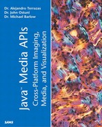
It turns out that there are numerous (almost infinite ways) to traverse kspace. One such trajectory is called spiral and benefits from improved coverage of kspace per unit time because of the inherent properties of the circle. The spiral kspace trajectory allows for images to be taken in snapshot (20ms) fashion and is used for such leading-edge applications such as imaging of the beating heart or imaging brain activity (functional magnetic resonance imaging). Figure 3.13 shows the final trajectory. Blue dots indicate that all time points up to the current time, whereas red dots indicate the full trajectory. This part of the visualization will be integrated with Java 3D models in the KspaceModeller application developed in Part III of this book.

In this example, we will use a slider bar to advance through time and see the current and previously sampled kspace points. The visualization will be made using an actual file that sits on the computer that runs an MRI scanner. We will later expand the number of kspace trajectories we can make, including making programmatic versions that aren't based on real data.

Step 1—The Visualization

First, let's make a skeleton of our external extended Canvas and call it KspaceCanvas. It is in this external class that all our painting will be accomplished. We will begin by painting an x- and y-axis with labels. An important part of this process is determining the height and width of the Canvas (accomplished with the getSize() method).

Listing 3.7 KspaceCanvas.java—a Custom Canvas for Visualization

import java.awt.*;
import java.awt.geom.*;
import java.awt.image.*;


public class KspaceCanvas extends Canvas {
   int xcenter, ycenter, offsetx, offsety;

   KspaceCanvas() {
    System.out.println("Creating an instance of KspaceCanvas");
   }

  public void drawKspace(int tpoint) {
      System.out.println("drawKspace");
      this.tpoint = tpoint;
      repaint();
   }

  public void paint(Graphics g){

      Graphics2D g2d = (Graphics2D)g;  //always!

       offsetx = (int) this.getSize().width/50;
       offsety = (int) this.getSize().height/50;
       xcenter = (int) this.getSize().width/2;
       ycenter = (int) this.getSize().height/2;

    //call method to paint the x-y axix
      paintAxis(g2d);
  }

   public void paintAxis(Graphics2D g2d) {
      //setup font for axis labeling
      Font f1 = new Font("TimesRoman", Font.BOLD, 14);
      g2d.setFont(f1);

      g2d.drawString("Kx",this.getSize().width-(2*offsetx),
                          this.getSize().height/2);

      g2d.drawString("Ky",this.getSize().width/2,offsetx);

      // draw  axis for kspace

      g2d.setColor(Color.black);  //set rendering attribute
      g2d.drawLine(offsetx, ycenter, xcenter-xoffset, ycenter-yoffset);
      g2d.drawLine(xcenter, yoffset, xcenter, ycenter-yoffset);

  }

}

Notice the drawKspace() method that receives the int argument tpoint, whose sole function is to set the current timepoint and call repaint(). The tpoint variable will represent the current timepoint in the kspace trajectory and will run from 0 to 5499. In the next step, we will create a slider bar with an attached listener. In that listener, the drawKspace() method will be called with the tpoint variable representing the current value of the slider bar.

The other important code for this part occurs in the overridden paint() and paintAxis() methods. First, in the paint() method, we get information necessary for scaling the axis appropriately. We want the x and y centers located half way up the Canvas regardless of size, so we use the getSize() method that was briefly described previously.

Step 2—Setting Up the User Interface

This step is fairly easy. We will extend JFrame and add two JPanels, one to hold the user interface components and another to hold our Canvas, as shown in Listing 3.8.

Listing 3.8 KspaceSpacePlot.java

import java.applet.Applet;
import java.awt.*;
import java.awt.event.*;
import javax.vecmath.*;
import javax.swing.*;
import java.awt.BorderLayout;

import java.util.Vector;

import java.awt.GraphicsConfiguration;

public class KspacePlot extends JFrame {

    int kwidth, kheight;

    KspaceData ks;
    KspaceCanvas kspacec;

  public KspacePlot (int initx, int inity) {

    super("Kspace Plot");

    Panel sliderpanel = new Panel();
    JSlider hslider = new JSlider();
    hslider.setMinimum(0);
    hslider.setMaximum(5498);
    hslider.setValue(0);
    hslider.setPreferredSize(new Dimension(300,20));
    sliderpanel.add(hslider);

    BorderLayout f1 = new BorderLayout();
    this.getContentPane().setLayout(f1);
    this.getContentPane().add(sliderpanel, BorderLayout.NORTH);
    ks = new KspaceData();
    kspacec = new KspaceCanvasA();

    this.getContentPane().add(kspacec);
    kspacec.drawKspace(0);
}

public static void main(String[] args) {
    int initialSizex=500;
    int initialSizey=500;

    WindowListener l = new WindowAdapter() {
     public void windowClosing(WindowEvent e)
        {System.exit(0);}
     public void windowClosed(WindowEvent e)
        {System.exit(0);}
     };

    KspacePlot k = new KspacePlot(initialSizex, initialSizey);
    k.addWindowListener(l);
    k.setSize(500,500);
    k.setVisible(true);

   }

}

class SliderListener implements ChangeListener {

   KspaceCanvasA kc;
   int slider_val;

   public SliderListener(KspaceCanvasA kc) {
        this.kc = kc;
   }

  public void stateChanged(ChangeEvent e) {

    JSlider s1 = (JSlider)e.getSource();
    slider_val = s1.getValue();
    System.out.println("Current value of the slider: " + slider_val);
    kc.drawKspace(

}//End of stateChanged
 }//End of SliderListener
//

Step 3—Reading the Scanner Trajectory

Because we want to plot an actual trajectory from the scanner, we will read bytes from a file into an array using a FileInputStream object. There are a few examples that read raw data in this book and you will find that, in practice, reading bytes is occasionally necessary. It probably isn't necessary to get into the details of this class. The important concept is that two files (kxtrap.flt and kytrap.flt) are read into two public arrays. Maximum and minimum values are computed for each array and stored in public variables. Another public array of time values is calculated based on the number of timepoints. The values stored in these arrays will be made accessible to KspaceCanvas by adding code to the KspaceCanvas constructor in “Step 4—Modifying KspaceCanvas to Plot the Data. ” Note that this class is external and stored in the file KspaceData.java (see Listing 3.9).

Listing 3.9 KspaceData.java—an External Class for Reading a Scanner Trajectory

import java.awt.*;
import java.io.*;

class KspaceData {

    int tpoints=5500;

    double Gxcoord[] = new double[tpoints];
    double Gycoord[] = new double[tpoints];
    int time[] = new int[tpoints];

    double Gx, Gy;

    double Gxmax=0.0;
    double Gymax=0.0;
    double Gxmin=0.0;
    double Gymin=0.0;

    KspaceData() {
       readdata();
    }

    public void readdata() {

     try {
            DataInputStream disx =
new DataInputStream(new FileInputStream("kxtrap.flt"));
            DataInputStream disy =
new DataInputStream(new FileInputStream("kytrap.flt"));

            try {
               for (int i=0; i < tpoints-1; i++) {
                   Gx = disx.readFloat();
           Gy = disy.readFloat();

             //find min and max gradient values to determine scaling
                   if (Gx > Gxmax) {
                      Gxmax=Gx;
                   }
                   if (Gy > Gymax) {
                       Gymax=Gy;
                   }
                  if (Gx < Gxmin) {
                      Gxmin=Gx;
                   }
                   if (Gy < Gymin) {
                       Gymin=Gy;
                   }

                   Gycoord[i] = Gy;
           Gxcoord[i] = Gx;
            }
            } catch (EOFException e) {
         }
         } catch (FileNotFoundException e) {
            System.out.println("DataIOTest: " + e);
        } catch (IOException e) {
            System.out.println("DataIOTest: " + e);
        }
   }

}

Step 4—Modifying KspaceCanvas to Plot the Data

Now that we can read the kx and ky files, it is time to plot the data over the axis that we made in step 1.

Add the method paintData() just below the paintAxis() method in KspaceCanvas.java:

//method to plot kspace data

public void paintData(Graphics2D g2d) {

    for (int i=1; i<tpoints-2; i++){
     // Scale Gx and Gy between -1 and 1; called Kx and Ky;
     // Multiply Kx and Ky times the width and height
     //of the Canvas in the same step
        Kx[i] = (ks.Kx[i] *this.getSize().width*scalefac;
        Ky[i] = (ks.Ky[i])*this.getSize().height*scalefac;

        g2d.setColor(Color.lightGray);
        g2d.draw(new Ellipse2D.Double(kxcenter + Kx[i],
                                      kycenter + Ky[i],3.0,3.0));
        g2d.setColor(Color.blue);
        g2d.fill(new Ellipse2D.Double(kxcenter + Kx[i],
                                      kycenter + Ky[i],4.0,4.0));

   }

}

In addition, we need to instantiate an object from our KspaceData class. In the KspacePlot.java class, add the following line just above the initial call to the KspaceCanvas constructor:

ks = new KspaceData();

We now need to modify the constructor to KspaceCanvas to allow for the passing in the newly constructed KspaceData object. First change the constructor in KspaceCanvas.java:

KspaceCanvas(KspaceData ks) {
    this.ks = ks;
}

And, change the initial call to the constructor in KspacePlot.java accordingly to the following:

kspacec = new KspaceCanvas(ks);

Finally, let's add the call to paintData() right after the call to paintAxis() in the paint() method of KspaceCanvas:

paintData(g2d);

After running the program, your screen should resemble Figure 3.8.

Step 5—Overriding the Update Method in KspaceCanvas

You will notice immediately that, although the program is starting to look promising, it is largely unusable in its present state. The primary problem is that the screen is erased and fully redrawn every time the slider bar changes.

Remember from before that repaint ends up calling update(), which puts the background color over the component before the Component's paint() method is called. This is one of the times when this is undesirable. We must therefore override the update() method and have our program only redraw the points that are new since the last call to repaint(). The following code segment is inserted into KspaceCanvas.java:

public void update(Graphics g) {
     paint(g);
}

Step 6—Add RenderingHints to Improve the Rendering

In this final step, we want to make the output look better. This is achieved through adding RenderingHints to the Graphics2D object. In this case, we want to add antialiasing so that our data point ellipses (dots) look smoother. We also need to add bicubic spline interpolation so that the dots line up better. Add the following lines in the paint() method:

RenderingHints interpHints =
              new RenderingHints(RenderingHints.KEY_INTERPOLATION,
                                 RenderingHints.VALUE_INTERPOLATION_BICUBIC);
g2d.setRenderingHints(interpHints);

RenderingHints antialiasHints =
              new RenderingHints(RenderingHints.KEY_ANTIALIASING,
                                 RenderingHints.VALUE_ANTIALIAS_ON);

g2d.setRenderingHints(antialiasHints);

You could just as well add this code to the constructor so that the RenderingHints aren't created each time paint() is called; however, this doesn't provide a substantial difference in performance.