Base R has a reputation for being slow and memory inefficient, a reputation that is at least somewhat earned. These faults are largely unnoticed on a modern PC for datasets of many thousands of records, but datasets with a million records or more can exceed the limits of what is currently possible with consumer-grade hardware. The problem is worsened if the dataset contains many features or if complex learning algorithms are being used.
Note
CRAN has a high-performance computing task view that lists packages pushing the boundaries on what is possible in R at http://cran.r-project.org/web/views/HighPerformanceComputing.html.
Packages that extend R past the capabilities of the base package are being developed rapidly. This work comes primarily on two fronts: some packages add the capability to manage extremely large datasets by making data operations faster or by allowing the size of data to exceed the amount of available system memory; others allow R to work faster, perhaps by spreading the work over additional computers or processors, by utilizing specialized computer hardware, or by providing machine learning optimized to big data problems.
Extremely large datasets can cause R to grind to a halt when the system runs out of memory to store the data. Even if the entire dataset can fit into the available memory, additional memory overhead is needed for data processing. Furthermore, very large datasets can take a long amount of time to process for no reason other than the sheer volume of records; even a quick operation can add up when performed many millions of times.
Years ago, many would suggest performing data preparation outside R in another programming language, then using R to perform analyses on a smaller subset of data. However, this is no longer necessary, as several packages have been contributed to R to address these big data problems.
The data.table package by Matt Dowle, Tom Short, Steve Lianoglou, and Arun Srinivasan provides an enhanced version of a data frame called a data table. The data.table objects are typically much faster than data frames for subsetting, joining, and grouping operations. And for the largest datasets—those with many millions of rows—these objects may be substantially faster than even dplyr objects. Yet, because a data.table object is essentially an improved data frame, the resulting objects can still be used by any R function that accepts a data frame.
Note
The data.table project can be found on GitHub at https://github.com/Rdatatable/data.table/wiki.
After installing the data.table package, the fread() function will read tabular files like CSVs into data table objects. For instance, to load the credit data used previously, type:
> library(data.table)
> credit <- fread("credit.csv")
The credit data table can then be queried using syntax similar to R's [row, col] form but optimized for speed and some additional useful conveniences. In particular, the data table structure allows the row portion to select rows using an abbreviated subsetting command, and the col portion to use a function that does something with the selected rows. For example, the following command computes the mean requested loan amount for people with a good credit history:
> credit[credit_history == "good", mean(amount)]
[1] 3040.958
By building larger queries with this simple syntax, very complex operations can be performed on data tables. And since the data structure is optimized for speed, it can be used with large datasets.
One limitation of data.table structures is that like data frames, they are limited by the available system memory. The next two sections discuss packages that overcome this shortcoming at the expense of breaking compatibility with many R functions.
Tip
The dplyr and data.table packages have unique strengths. For an in-depth comparison, see the following Reddit discussion at https://www.reddit.com/r/rstats/comments/acjr9d/dplyr_performance/ and a similar conversation on Stack Overflow: https://stackoverflow.com/questions/21435339/data-table-vs-dplyr-can-one-do-something-well-the-other-cant-or-does-poorly. It is also possible to have the best of both worlds, as data.table structures can be loaded into dplyr using the tbl_dt() function.
The ff package by Daniel Adler, Christian Gläser, Oleg Nenadic, Jens Oehlschlägel, and Walter Zucchini provides an alternative to a data frame (ffdf) that allows datasets of over two billion rows to be created, even if this far exceeds the available system memory.
The ffdf structure has a physical component that stores the data on disk in a highly efficient form and a virtual component that acts like a typical R data frame but transparently points to the data stored in the physical component. You can imagine the ffdf object as a map that points to a location of data on a disk.
Note
The ff project is on the web at http://ff.r-forge.r-project.org/.
A downside of ffdf data structures is that they cannot be used natively by most R functions. Instead, the data must be processed in small chunks, and the results should be combined later on. The upside of chunking the data is that the task can be divided across several processors simultaneously using the parallel computing methods presented later in this chapter.
After installing the ff package, to read in a large CSV file use the read.csv.ffdf() function as follows:
> library(ff)
> credit <- read.csv.ffdf(file = "credit.csv", header = TRUE)
Unfortunately, we cannot work directly with the ffdf object, as attempting to treat it like a traditional data frame results in an error message:
> mean(credit$amount)
[1] NA
Warning message:
In mean.default(credit$amount) :
  argument is not numeric or logical: returning NA
The ffbase package by Edwin de Jonge, Jan Wijffels, and Jan van der Laan addresses this issue somewhat by adding capabilities for basic analyses using ff objects. This makes it possible to use ff objects directly for data exploration. For instance, after installing the ffbase package, the mean function works as expected:
> library(ffbase)
> mean(credit$amount)
[1] 3271.258
The package also provides other basic functionality such as mathematical operators, query functions, summary statistics, and wrappers for working with optimized machine learning algorithms like biglm (described later in this chapter). Though these do not completely eliminate the challenges of working with extremely large datasets, they make the process a bit more seamless.
Note
For more information about advanced functionality, visit the ffbase project site at http://github.com/edwindj/ffbase.
The bigmemory package by Michael J. Kane, John W. Emerson, and Peter Haverty allows extremely large matrices that exceed the amount of available system memory. The matrices can be stored on disk or in shared memory, allowing them to be used by other processes on the same computer or across a network. This facilitates parallel computing methods, such as those covered later in this chapter.
Note
Additional documentation on the bigmemory package can be found at http://www.bigmemory.org/.
Because bigmemory matrices are intentionally unlike data frames, they cannot be used directly with most of the machine learning methods covered in this book. They also can only be used with numeric data. That said, since they are similar to a typical R matrix, it is easy to create smaller samples or chunks that can be converted to standard R data structures.
The authors also provide bigalgebra, biganalytics, and bigtabulate packages, which allow simple analyses to be performed on the matrices. Of particular note is the bigkmeans() function in the biganalytics package, which performs k-means clustering as described in Chapter 9, Finding Groups of Data – Clustering with k-means. Due to the highly specialized nature of these packages, use cases are outside the scope of this chapter.
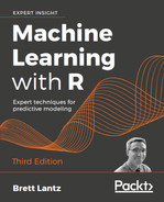
In the early days of computing, processors executed instructions in serial, which meant that they were limited to performing a single task at a time. The next instruction could not be started until the previous instruction was complete. Although it was widely known that many tasks could be completed more efficiently by completing steps simultaneously, the technology simply did not exist yet.
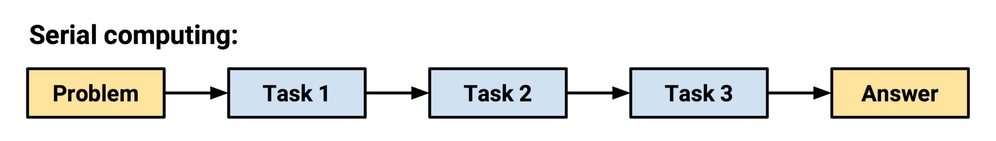
Figure 12.5: In serial computing, tasks cannot begin until prior tasks have completed
This was addressed by the development of parallel computing methods, which use a set of two or more processors or computers to solve a larger problem. Many modern computers are designed for parallel computing. Even in the case that they have a single processor, they often have two or more cores that are capable of working in parallel. This allows tasks to be accomplished independently from one another.
Figure 12.6: In parallel computing, tasks occur simultaneously. Their results must be combined at the end.
Networks of multiple computers called clusters can also be used for parallel computing. A large cluster may include a variety of hardware and be separated over large distances. In this case, the cluster is known as a grid. Taken to an extreme, a cluster or grid of hundreds or thousands of computers running commodity hardware could be a very powerful system.
The catch, however, is that not every problem can be parallelized. Certain problems are more conducive to parallel execution than others. One might expect that adding 100 processors would result in 100 times the work being accomplished in the same amount of time (that is, the overall execution time is 1/100), but this is typically not the case. The reason is that it takes effort to manage the workers. Work must be divided into equal, non-overlapping tasks, and each of the workers' results must be combined into one final answer.
So-called embarrassingly parallel problems are the ideal. These tasks are easy to reduce into non-overlapping blocks of work, and the results are easy to recombine. An example of an embarrassingly parallel machine learning task would be 10-fold cross-validation; once the 10 samples are divided, each of the 10 blocks of work is independent, meaning that they do not affect the others. As you will soon see, this task can be sped up quite dramatically using parallel computing.
Efforts to speed up R will be wasted if it is not possible to systematically measure how much time was saved. Although a stopwatch is one option, an easier solution is to wrap the offending code in a system.time() function.
For example, on the author's laptop, the system.time() function notes that it takes about 0.080 seconds to generate a million random numbers:
> system.time(rnorm(1000000))
   user  system elapsed
  0.079   0.000   0.067
The same function can be used for evaluating improvement in performance, obtained with the methods that were just described or any R function.
Note
For what it's worth, when the first edition of this book was published, generating a million random numbers took 0.130 seconds; the same took about 0.093 seconds for the second edition. Here it takes about 0.067 seconds. Although I've used a slightly more powerful computer each time, this reduction of about 50 percent of the processing time over the course of about six years illustrates just how quickly computer hardware and software are improving.
The parallel package, included with R version 2.14.0 and later, has lowered the entry barrier to deploying parallel algorithms by providing a standard framework for setting up worker processes that can complete tasks simultaneously. It does this by including components of the multicore and snow packages, which each take a different approach to multitasking.
If your computer is reasonably recent, you are likely to be able to use parallel processing. To determine the number of cores your machine has, use the detectCores() function as follows. Note that your output will differ depending on your hardware specifications:
> library(parallel)
> detectCores()
[1] 8
The multicore package was developed by Simon Urbanek and allows parallel processing on a single machine that has multiple processors or processor cores. It utilizes the multitasking capabilities of a computer's operating system to fork additional R sessions that share the same memory, and is perhaps the simplest way to get started with parallel processing in R. Unfortunately, because Windows does not support forking, this solution will not work everywhere.
An easy way to get started with the multicore functionality is to use the mclapply() function, which is a multi-core version of lapply(). For instance, the following blocks of code illustrate how the task of generating a million random numbers can be divided across 1, 2, 4, and 8 cores. The unlist() function is used to combine the parallel results (a list) into a single vector after each core has completed its chunk of work:
> system.time(l1 <- unlist(mclapply(1:10, function(x) {
+   rnorm(1000000)}, mc.cores = 1)))
   user  system elapsed
  0.627   0.015   0.647

> system.time(l2 <- unlist(mclapply(1:10, function(x) {
+   rnorm(1000000)}, mc.cores = 2)))
   user  system elapsed
  0.751   0.211   0.568

> system.time(l4 <- unlist(mclapply(1:10, function(x) {
+   rnorm(1000000) }, mc.cores = 4)))
   user  system elapsed
  0.786   0.270   0.405

> system.time(l8 <- unlist(mclapply(1:10, function(x) {
+   rnorm(1000000) }, mc.cores = 8)))
   user  system elapsed
  1.033   0.315   0.321
Notice how as the number of cores increases, the elapsed time decreases, though the benefit tapers off. Though this is a simple example, it can be adapted easily to many other tasks.
The snow package (simple networking of workstations) by Luke Tierney, A. J. Rossini, Na Li, and H. Sevcikova allows parallel computing on multicore or multiprocessor machines as well as on a network of multiple machines. It is slightly more difficult to use, but offers much more power and flexibility. The snow functionality is included in the parallel package, so to set up a cluster on a single machine, use the makeCluster() function with the number of cores to be used:
> cl1 <- makeCluster(4)
Because snow communicates via network traffic, depending on your operating system, you may receive a message to approve access through your firewall.
To confirm the cluster is operational, we can ask each node to report back its hostname. The clusterCall() function executes a function on each machine in the cluster. In this case, we'll define a function that simply calls the Sys.info() function and returns the nodename parameter:
> clusterCall(cl1, function() { Sys.info()["nodename"] } )
[[1]]
                  nodename
"Bretts-Macbook-Pro.local"

[[2]]
                  nodename
"Bretts-Macbook-Pro.local"

[[3]]
                  nodename
"Bretts-Macbook-Pro.local"

[[4]]
                  nodename
"Bretts-Macbook-Pro.local"
Unsurprisingly, since all four nodes are running on a single machine, they report back the same hostname. To have the four nodes run a different command, supply them with a unique parameter via the clusterApply() function. Here, we'll supply each node with a different letter. Each node will then perform a simple function on its letter in parallel:
> clusterApply(cl1, c('A', 'B', 'C', 'D'),
               function(x) { paste("Cluster", x, "ready!") })
[[1]]
[1] "Cluster A ready!"

[[2]]
[1] "Cluster B ready!"

[[3]]
[1] "Cluster C ready!"

[[4]]
[1] "Cluster D ready!"
When we're done with the cluster, it's important to terminate the processes it spawned. This will free up the resources each node is using:
> stopCluster(cl1)
Using these simple commands, it is possible to speed up many machine learning tasks. For the largest big data problems, much more complex snow configurations are possible. For instance, you may attempt to configure a Beowulf cluster—a network of many consumer-grade machines. In academic and industry research settings with dedicated computing clusters, snow can use the Rmpi package to access these high-performance message passing interface (MPI) servers. Working with such clusters requires knowledge of network configurations and computing hardware outside the scope of this book.
Note
For a much more detailed introduction to snow, including some information on how to configure parallel computing on several computers over a network, see the following lecture by Luke Tierney: http://homepage.stat.uiowa.edu/~luke/classes/295-hpc/notes/snow.pdf.
The foreach package by Rich Calaway and Steve Weston provides perhaps the easiest way to get started with parallel computing, especially if you are running R on the Windows operating system, as some of the other packages are platform-specific.
The core of the package is a foreach looping construct. If you have worked with other programming languages, this may be familiar. Essentially, it allows looping over a number of items in a set, without explicitly counting the number of items; in other words, for each item in the set, do something.
If you're thinking that R already provides a set of apply functions to loop over sets of items (for example, apply(), lapply(), sapply(), and so on), you are correct. However, the foreach loop has an additional benefit: iterations of the loop can be completed in parallel using a very simple syntax. Let's see how this works.
Recall the command we've been using to generate a million random numbers. To make this more challenging, let's increase the count to a hundred million, which causes the process to take over six seconds:
> system.time(l1 <- rnorm(100000000))
   user  system elapsed
  5.873   0.204   6.087
After the foreach package has been installed, the same task can be expressed by a loop that generates four sets of 25,000,000 random numbers. The .combine parameter is an optional setting that tells foreach which function it should use to combine the final set of results from each loop iteration. In this case, since each iteration generates a set of random numbers, we simply use the c() concatenate function to create a single, combined vector:
> library(foreach)
> system.time(l4 <- foreach(i = 1:4, .combine = 'c')
                %do% rnorm(25000000))
   user  system elapsed
  6.177   0.391   6.578
If you noticed that this function didn't result in a speed improvement, good catch! In fact, the process was actually slower. The reason is that by default, the foreach package runs each loop iteration in serial, and the function adds a small amount of computational overhead to the process. The sister package doParallel provides a parallel backend for foreach that utilizes the parallel package included with R, described earlier in this chapter. After installing the doParallel package, simply register the number of cores and swap the %do% command with %dopar% as follows:
> library(doParallel)
> registerDoParallel(cores = 4)
> system.time(l4p <- foreach(i = 1:4, .combine = 'c')
                       %dopar% rnorm(25000000))
   user  system elapsed
  7.841   2.288   3.894
As shown in the output, this results in the expected performance increase, cutting the execution time by about 40 percent.
To close the doParallel cluster, simply type:
> stopImplicitCluster()
Though the cluster will be closed automatically at the conclusion of the R session, it is better form to do so explicitly.
The caret package by Max Kuhn (covered extensively in Chapter 10, Evaluating Model Performance and Chapter 11, Improving Model Performance) will transparently utilize a parallel backend if one has been registered with R using the foreach package described previously.
Let's take a look at a simple example in which we attempt to train a random forest model on the credit dataset. Without parallelization, the model takes about 79 seconds to train:
> library(caret)
> credit <- read.csv("credit.csv")
> system.time(train(default ~ ., data = credit, method = "rf"))
   user  system elapsed
 77.345   1.778  79.205
On the other hand, if we use the doParallel package to register four cores to be used in parallel, the model takes under 20 seconds to build—less than a quarter of the time—and we didn't need to change even a single line of caret code:
> library(doParallel)
> registerDoParallel(cores = 8)
> system.time(train(default ~ ., data = credit, method = "rf"))
   user  system elapsed
122.579   3.292  19.034
Many of the tasks involved in training and evaluating models, such as creating random samples and repeatedly testing predictions for 10-fold cross-validation are embarrassingly parallel and ripe for performance improvements. With this in mind, it is wise to always register multiple cores before beginning a caret project.
Note
Configuration instructions and a case study of the performance improvements for enabling parallel processing in caret are available at the project's website: http://topepo.github.io/caret/parallel.html.
The MapReduce programming model was developed at Google as a way to process its data on a large cluster of networked computers. MapReduce defined parallel programming as a two-step process:
A popular open-source alternative to the proprietary MapReduce framework is Apache Hadoop. The Hadoop software comprises of the MapReduce concept plus a distributed filesystem capable of storing large amounts of data across a cluster of computers.
Note
Packt Publishing has published a large number of books on Hadoop. To search current offerings, visit https://www.packtpub.com/all/?search=hadoop.
Several R projects that provide an R interface to Hadoop are in development. The RHadoop project by Revolution Analytics provides an R interface to Hadoop. The project provides a package, rmr2, intended to be an easy way for R developers to write MapReduce programs. Another companion package, plyrmr, provides functionality similar to the dplyr package for processing large datasets. Additional RHadoop packages provide R functions for accessing Hadoop's distributed data stores.
Note
For more information about the RHadoop project, see https://github.com/RevolutionAnalytics/RHadoop/wiki.
Although Hadoop is a mature framework, it requires somewhat specialized programming skills to take advantage of its capabilities and to perform even basic machine learning tasks. Perhaps this explains its apparent lack of popularity with R users. Additionally, although Hadoop is excellent at working with extremely large amounts of data, it may not always be the fastest option because it keeps all data on disk rather than utilizing available memory. The next section covers an extension to Hadoop that addresses these speed and usability issues.
The Apache Spark project is a cluster-computing framework for big data, offering many advantages over Apache Hadoop. Because it takes advantage of the cluster's available memory, it can process data approximately 100x faster than Hadoop. Additionally, it provides high-level libraries for many common data processing, analysis, and modeling tasks. These include the SparkSQL data query language, the MLlib machine learning library, GraphX for graph and network analysis, and the Spark Streaming library for processing real-time data streams.
Note
Packt Publishing has published a large number of books on Spark. To search current offerings, visit https://www.packtpub.com/all/?search=spark.
Apache Spark is often run remotely on a cloud-hosted cluster of virtual machines, but its benefits can also be seen running on your own hardware. In either case, the sparklyr package connects to the cluster and provides a dplyr interface for analyzing the data using Spark. More detailed instructions for using Spark with R can be found at https://spark.rstudio.com, but the basics of getting up-and-running are fairly straightforward.
To illustrate the fundamentals, let's build a random forest model on the credit dataset to predict loan defaults. We'll begin by installing the sparklyr package. Then, you can instantiate a Spark cluster on your local machine using the following code:
> install.packages("sparklyr")
> library(sparklyr)
> spark_install(version = "2.1.0")
> spark_cluster <- spark_connect(master = "local")
Next, we'll load the loan dataset from the credit.csv file on our local machine into the Spark instance, then use the Spark data frame partitioning function sdf_partition() to randomly assign 75 and 25 percent of data to training and test sets. The seed parameter is the random seed to ensure the results are identical each time this code is run:
> credit_spark <- spark_read_csv(spark_cluster, "credit.csv")

> splits <- sdf_partition(credit_spark,
                          train = 0.75, test = 0.25,
                          seed = 123)
Lastly, we'll pipe the training data into the random forest model function, make predictions, and use the classification evaluator to compute the AUC on the test set:
> credit_rf <- splits$train %>%
    ml_random_forest(default ~ .)
> pred <- ml_predict(credit_rf, splits$test)
> ml_binary_classification_evaluator(pred,
    metric_name = "areaUnderROC")
[1] 0.7848068
With just a few lines of R code, we've built a random forest model using Spark that could expand to model millions of records. If even more computing power is needed, the code can be run in the cloud using a massively parallel Spark cluster simply by pointing the spark_connect() function to the correct hostname. The code can also be easily adapted to other modeling approaches using one of the supervised learning functions listed at https://spark.rstudio.com/mlib/.
Tip
Perhaps the easiest way to get started using Spark is with Databricks, a cloud platform developed by the creators of Spark that makes it easy to manage and scale clusters via a web-based interface. The free "community edition" provides a small cluster for you to try a number of tutorials or even experiment with your own data. Check it out at https://databricks.com.
Some of the machine learning algorithms covered in this book are able to work on extremely large datasets with relatively minor modifications. For instance, it would be fairly straightforward to implement Naive Bayes or the Apriori algorithm using one of the data structures for big datasets described in the previous sections. Some types of learners, such as ensembles, lend themselves well to parallelization because the work of each model can be distributed across processors or computers in a cluster. On the other hand, some require larger changes to the data or algorithm, or need to be rethought altogether before they can be used with massive datasets.
The following sections examine packages that provide optimized versions of the learning algorithms we've worked with so far.
The biglm package by Thomas Lumley provides functions for training regression models on datasets that may be too large to fit into memory. It works by an iterative process in which the model is updated little by little using small chunks of data. In spite of the different approach, the results will be nearly identical to what would have been obtained running the conventional lm() function on the entire dataset.
For convenience when working with the largest datasets, the biglm() function allows the use of a SQL database in place of a data frame. The model can also be trained with chunks obtained from data objects created by the ff package described previously.
The ranger package by Marvin N. Wright, Stefan Wager, and Philipp Probst is a faster implementation of the random forest algorithm, particularly for datasets with a large number of features or examples. The function is used much like the earlier random forest:
> library(ranger)
> credit <- read.csv("credit.csv")

> m <- ranger(default ~ ., data = credit,
              num.trees = 500,
              mtry = 4)

> p <- predict(m, credit)
Note that unlike most of the predict() results used previously, the ranger predictions are stored as a sub-object in the prediction object:
> head(p$predictions)
[1] no  yes no  no  yes no
Levels: no yes
Using the ranger() function is the easiest way to build bigger and better random forests, without resorting to cluster computing or alternative data structures.
The bigrf package by Aloysius Lim implements the training of random forests for classification and regression on datasets that are too large to fit into memory using bigmemory objects as described earlier in this chapter. For speedier forest growth, the package can be used with the foreach and doParallel packages described previously to grow trees in parallel.
Note
For more information, including examples and Windows installation instructions, see the package wiki hosted at https://github.com/aloysius-lim/bigrf.
The H2O project is a big data framework that provides fast in-memory implementations of machine learning algorithms, which can also operate in a cluster computing environment. It includes functions for many of the methods covered in this book, including Naive Bayes, regression, deep neural networks, k-means clustering, ensemble methods, and random forests, among many others.
H2O uses heuristics to find approximate solutions to machine learning problems by iterating repeatedly over smaller chunks of the data. This gives the user the control to determine exactly how much of a massive dataset the learner should use. For some problems, a quick solution may be acceptable, but for others, the complete set may be required, which will require additional training time.
H2O is usually substantially faster and performs better on very massive datasets relative to Apache Spark's machine learning functions (MLlib), which itself is often much faster than base R. However, because Apache Spark is a commonly used cluster computing and big data preparation environment, H2O can be run on Apache Spark using the Sparkling Water software. With Sparkling Water, data scientists have the best of both worlds—the benefits of Spark for data preparation, and the benefits of H2O for machine learning.
The h2o package provides functionality for accessing an H2O instance from within the R environment. A full tutorial on H2O is outside the scope of this book, and documentation is available at http://docs.h2o.ai, but the basics are straightforward. To get started, install and load the h2o package. Then, initialize a local H2O instance using the following code:
> library(h2o)
> h2o_instance <- h2o.init()
This starts an H2O server on your computer, which can be viewed via H2O Flow at http://localhost:54321. The H2O Flow web application allows you to administer and send commands to the H2O server, or even build and evaluate models using a simple, browser-based interface:

Figure 12.7: H2O Flow is a web application for interacting with the H2O instance
Although you could complete an analysis within this interface, let's go back to R and use H2O on the loan default data that we examined previously. First, we need to upload the credit.csv dataset to this instance using the following command:
> credit.hex <- h2o.uploadFile("credit.csv")
Note that the .hex extension is used for referring to an H2O data frame.
Next, we'll apply H2O's random forest implementation to this dataset using the following command:
> h2o.randomForest(y = "default",
                   training_frame = credit.hex,
                   ntrees = 500,
                   seed = 123)
The output of this command includes information on the out-of-bag estimates of model performance:
** Reported on training data. **
** Metrics reported on Out-Of-Bag training samples **

MSE:  0.1636964
RMSE:  0.4045941
LogLoss:  0.4956524
Mean Per-Class Error:  0.2835714
AUC:  0.7844881
pr_auc:  0.6192192
Gini:  0.5689762
Although the credit dataset used here is not very large, the H2O code used here would scale to datasets of almost any size. Additionally, the code would be virtually unchanged if it were to be run in the cloud—simply point the h2o.init() function to the remote host.
An alternative to parallel processing uses a computer's graphics processing unit (GPU) to increase the speed of mathematical calculations. A GPU is a specialized processor that is optimized for rapidly displaying images on a computer screen. Because a computer often needs to display complex 3D graphics (particularly for video games), many GPUs use hardware designed for parallel processing and extremely efficient matrix and vector calculations. A side benefit is that they can be used for efficiently solving certain types of mathematical problems. Where a typical laptop or desktop computer processor may have up to 16 cores, a typical GPU may have thousands or even tens of thousands.

Figure 12.8: A graphics processing unit (GPU) has many times more cores than the typical central processing unit (CPU)
The downside of GPU computing is that it requires specific hardware that is not included with many computers. In most cases, a GPU from the manufacturer NVIDIA is required, as it provides a proprietary framework called Complete Unified Device Architecture (CUDA) that makes the GPU programmable using common languages such as C++.
Note
For more information on NVIDIA's role in GPU computing, go to https://www.nvidia.com/en-us/about-nvidia/ai-computing/.
The gputools package by Josh Buckner, Mark Seligman, and Justin Wilson implements several R functions, such as matrix operations, clustering, and regression modeling using the NVIDIA CUDA toolkit. The package requires a CUDA 1.3 or higher GPU and the installation of the NVIDIA CUDA toolkit.
One of the most significant recent innovations in machine learning software is TensorFlow (https://www.tensorflow.org), an open-source mathematical library developed at Google for advanced machine learning. TensorFlow provides a computing interface using directed graphs that "flow" data arrays called tensors through a number of mathematical operations. In this way, a very complex "black box" method like a deep neural network can be represented as a simpler abstraction. Additionally, because the graph stores the set of computations as a set of dependent steps, TensorFlow is able to distribute the work across available CPU or GPU cores and take advantage of massively parallel computing environments.
Note
Packt Publishing has published a large number of books on TensorFlow. To search current offerings, visit https://www.packtpub.com/all/?search=tensorflow.
R interfaces to TensorFlow have been developed by the team at RStudio. The tensorflow package provides access to the core API, while the tfestimators package provides access to higher-level machine learning functionality. Note that TensorFlow's directed graph approach can be used to implement many different machine learning models, including many of the ones discussed in this book. However, to do so requires a thorough understanding of the matrix mathematics that define each model, and thus is well outside the scope of this text. For more information about these packages and RStudio's ability to interface with TensorFlow, visit https://tensorflow.rstudio.com.
Tip
Due to TensorFlow's unique approach to estimating machine learning models, you may find vast differences in the terminology used by its practitioners, even for simpler methods like linear regression. You may hear phrases like "cost function," "gradient descent," and "optimization." This terminology reflects the fact that machine learning with TensorFlow is in many ways analogous to building a neural network that finds the best approximation of the desired model.
Because the computing framework provided by TensorFlow is ideal for constructing deep neural networks, the Keras library (https://keras.io) was developed to provide a simpler, high-level interface to this widely-used functionality. Keras was developed in Python, and can use TensorFlow or similar frameworks as the backend computing engine. Using Keras, it is possible to do deep learning in just a few lines of code—even for challenging applications such as image classification.
Note
Packt Publishing offers a number of books and videos to learn Keras. To search current offerings, visit https://www.packtpub.com/all/?search=keras.
The keras package, developed by RStudio CEO and founder J.J. Allaire, provides an R interface to Keras. Although there is very little code required to use the keras package, developing useful deep learning models requires extensive knowledge of neural networks as well as familiarity with TensorFlow and the Keras API. Additionally, to build anything but the simplest neural networks, it is essential to use a GPU—the code will simply never finish running without the massively-parallel processing the GPU provides. For these reasons, a tutorial is outside the scope of this book. Instead, refer to the RStudio documentation at https://keras.rstudio.com, or the book Deep Learning with R (2018), which was co-authored by Francois Chollet and J.J. Allaire—the creators of Keras and the keras package, respectively. Given their credentials, there is no better place to begin learning about this tool.
Tip
At the time of publication, a typical GPU used for deep learning is priced at several hundred US dollars for entry-level models and around $1,000-$3,000 for moderately-priced units with greater performance. High-end units may cost many thousands of dollars. Rather than spend this much up front, many people rent server time by the hour on cloud providers like Amazon AWS and Microsoft Azure, where it costs approximately $1 per hour for a minimal GPU instance—just don't forget to shut it down when your work completes, as it can get expensive quite quickly! The RStudio team also provides information about their preferred host at https://tensorflow.rstudio.com/tools/cloud_desktop_gpu.html.