9
Theories of Consumption
After studying this topic, you should be able to understand
- The basic principle of absolute income hypothesis is that the individual consumer will determine the fraction of his current income that he will allocate to consumption on the basis of his absolute income level.
- According to the relative income hypothesis, the fraction of a family’s income that will be allocated to consumption will depend on its income level relative to the income level of the other families with which it classifies itself.
- The permanent income hypothesis puts forward the view that consumption is related to the permanent income.
- The average propensity to consume, expressed in terms of the permanent income, is the same on an average for all families whether rich or poor.
- The life cycle hypothesis puts forward the view that consumption is related to the present value of the individual’s income or wealth.
- Besides income, there are many other factors like the rate of interest, price level, price expectations, income distribution and financial assets, which influence the consumption levels.
INTRODUCTION
In Chapter 5, we had introduced the relationship between consumption and income in a simplified form. This chapter analyses the relationship more closely by looking at four hypotheses, which focus on the influence of income on consumption, namely, the absolute income hypothesis, relative income hypothesis, permanent income hypothesis and the life cycle hypothesis.
It was with Keynes’ theory of the consumption function that optimism was felt that perhaps it was possible to predict consumption expenditures. However, this optimism was short lived and the predictions in the post World War II period proved to be off the mark. Hence, economists came up with different theories to explain the factors, which in addition to income, determine the consumption expenditures. These factors could range from age size of the family, demographic characteristics, wealth, and rate of interest to the income distribution.
ABSOLUTE INCOME HYPOTHESIS
The absolute income hypothesis is associated with Keynes and later with James Tobin and Arthur Smithies. The basic principle of this hypothesis is that the individual consumer will determine the fraction of his current income that he will allocate to consumption on the basis of his absolute income level. Thus, the individual consumer’s consumption expenditure depends on his absolute income level. Everything else remaining unchanged, an increase in the income will lead to a decrease in the fraction of the income allocated to consumption.
The basic principle of absolute income hypothesis is that the individual consumer will determine the fraction of his current income that he will allocate to consumption on the basis of his absolute income level.
The study of the relationship between consumption and income has gained importance in the last 10 to 15 years. It has created interest among sociologists, anthropologists, historians and philosophers also. However, in spite of the vital role played by consumption in economic theory, economists have not contributed much in the new wave of research which has accompanied the dynamic changes in this field. This is a reflection of the rigidity in the conventional theory of consumer behaviour. This theory assumes that consumption depends on income, prices and tastes only. It is not in any way influenced by the culture, society, economic institutions and the choices of the others. Hence, economists feel that there is little point in discussing any of these other social factors which are said to influence consumption.
Figure 9.1 depicts the relationship between income and consumption as in the absolute income hypothesis.
The straight line through the axis is the 45° line showing the hypothetical relationship between consumption and income that the current consumption is always equal to the current income. Thus, when income is zero consumption is always zero.
The curve C illustrates Keynes’ absolute income hypothesis. It can be analysed in three parts:
- Until point E on the curve C corresponding to the income level before Y1, the consumption expenditure exceeds the current income level. This clearly shows that families with low incomes have a high marginal propensity to consume as they spend a large proportion of their incomes on consumption.
- At point E on the curve C corresponding to the income level Y1, the consumption expenditure equals the current income level.
Thus, current consumption and current income break even at the income Y1.
- Beyond point E on the curve C corresponding to the income level greater than Y1, the consumption expenditure is less than the current income level. Hence, the consumption increases with income but at a lesser rate. This explains why families with high incomes have a low marginal propensity to consume as they spend a small proportion of their incomes on consumption and save a larger proportion of their incomes.
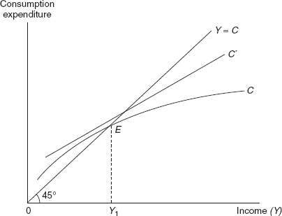
Figure 9.1 Relationship Between Income and Consumption: The Absolute Income Hypothesis
The above analysis gives rise to an income consumption curve, which is upward sloping but with a downwards bend.
Some conclusions, which can be drawn, are:
- The high income families save a large proportion of their incomes as compared to the low income families as they are left with a large proportion of their incomes after fulfilling their consumption needs. Thus, the marginal propensity to consume of high income groups will be low.
- As families climb up the income scale, the proportion of income that they can save increases.
- For the average family, there is a decrease in the average propensity to consume when it climbs up the income scale.
In the initial years, the absolute income hypothesis was widely accepted. Later on, the Keynesians modified the relationship.
Criticisms: The absolute income hypothesis assumes that there is no change in any of the factors that influence consumption, which is incorrect. Also, as already mentioned, empirical data in the post World War II period does not support Keynes’ absolute income hypothesis. Yet, we cannot deny the importance of Keynes’ work which marked the beginning of an era due to which attempts were made and researches were conducted to analyse the relationship between consumption and income, which initiated the different theories which came up post Keynes.
RECAP
- Everything else remaining unchanged, an increase in the income will lead to a decrease in the fraction of the income allocated to consumption.
- Families with high incomes have a low marginal propensity to consume.
RELATIVE INCOME HYPOTHESIS
The ‘relative income hypothesis’ was put forward by J. S. Duesenberry in the 1940s. According to this hypothesis, the fraction of a family’s income that will be allocated to consumption will depend on its income level relative to the income level of the other families (with which it classifies itself) and not on its absolute income level. Thus,
- If a family’s absolute income increases but its relative income (income relative to the other families with which it classifies itself) remains unchanged, then its distribution of income between consumption and savings will also remain unchanged. There will be an increase in the absolute consumption. But, the fraction of the family’s income that is allocated to consumption will remain the same.
- If a family’s income remains the same, but its relative income (income relative to the other families with which it classifies itself) deteriorates because there occurs an increase in the income of the other families with which it classifies itself, then there will be a change in the family’s distribution of income between consumption and savings. Not only will there be an increase in the absolute consumption, but the fraction of the family’s income that is allocated to consumption will also increase. Thus, even though there has been no change in the absolute income, the fraction of the family’s income that is devoted to consumption increases.
The ‘relative income hypothesis’ lays emphasis on the emulative nature of a family. A family with a certain given income will spend a larger fraction of its income on consumption if it is living in a community in which that income is considered to be low as compared to a community in which that income is considered to be high. This is due to what Duesenberry called the ‘demonstration effect’ where families are influenced by the other family’s standard of living and thus try to ‘keep up with the Joneses’. Hence, the absolute income becomes less important and the family’s relative income in the community that it lives in becomes more important.
In Figure 9.1, suppose that there is a doubling-up of the absolute incomes of all the families between a certain time period. It is important to note that this does not lead to any change in the distribution of the income. Hence, the relative position of each family on the income scale remains unchanged. According to the relative income hypothesis, for the average family there will be no change in the fraction of the income devoted to consumption. Thus as long as the relative income remains unchanged, the fraction of a family’s income devoted to consumption will also remain unchanged, even though there may be a change in the family’s absolute income.
Each family will, thus, move along the consumption function C′ in Figure 9.1 which is a straight line depicting that the fraction of income devoted to consumption remains unchanged. Hence, the average propensity to consume will remain the same before and after the change in the income. An average family will not feel that it is better off as its relative position on the income scale has not changed and thus it will continue to consume the same proportion of its income that it was consuming earlier. Hence, its average propensity to consume will remain as earlier and it will not move along the curve C as predicted by the absolute income hypothesis where as the family’s absolute income increases there is a decrease in the average propensity to consume.
Similar to the absolute income hypothesis, the relative income hypothesis also assumes that there is no change in any of the factors which influence consumption.
Criticisms
- According to the relative income hypothesis, upward changes in income and consumption are proportional where as empirical evidence suggests that unexpected gains in the income levels are linked to less than proportional increases in consumption levels.
- The view that consumption standards once maintained are permanent and thus irreversible is also not correct.
RECAP
- The ‘relative income hypothesis’ lays emphasis on the emulative nature of a family.
PERMANENT INCOME HYPOTHESIS
The permanent income hypothesis was developed by Milton Friedman in 1957. It is a departure from the earlier two analyses in that it focused on the concept of the permanent income. It puts forward the view that consumption is related to the permanent income. The absolute income hypothesis and the relative income hypothesis related consumption to the individual family’s current income. Both the absolute and relative incomes are current incomes.
A family’s permanent income is not in any way indicated by its current income. It is, in fact, determined by the expected income over the next few years and is thus a long-term estimate of income. It is determined by the family’s wealth, both physical and human wealth. Thus the permanent income is the average income, which is regarded as permanent by the individual family. It will determine the steady pace of expenditure, which the family could maintain for the rest of their life.
The family’s measured income or the observed income may be different from the permanent income. Friedman has split up the measured income into two components, the permanent income and the transitory income. The difference between the measured income and the permanent income is, thus, related to whether the transitory income is positive or negative, that is:
- If a wage earner in a family receives an unexpected bonus in a particular year, then in that case the transitory income is positive and thus the measured income is greater than the permanent income.
- If a wage earner in a family suffers an unanticipated loss in his income in a particular year, say due to a fire, then in that case the transitory income is negative and thus the measured income is lesser than the permanent income.
Friedman has similarly split up consumption into two components, permanent consumption and transitory consumption. Permanent income is what households expect to receive over a certain period in the future where as the transitory income forms the unanticipated addition or subtraction in the permanent income. His main argument is that permanent consumption depends on the permanent income. In fact, it is a constant fraction of the permanent income. Permanent consumption is determined by different factors like the ratio of human wealth to the total wealth, the rate of interest and tastes which are influenced by factors like age and the composition of the family. If these factors do not vary much, then in that case, the average ratio of consumption to the permanent income will turn out to be the same even for families at different income levels. According to the hypothesis, the average fraction of the permanent income of a family that is allocated to consumption is the same whether they are at the top or the bottom of the income scale, or in other words, whether they are rich or poor. Thus the average propensity to consume expressed in terms of the permanent income is the same on an average for all families, whether rich or poor.
The above analysis implies that the average propensity to save, when expressed in terms of the permanent income, is the same for all families whether rich or poor. The main purpose of saving is to provide for the future by smoothening out consumption over a period of time. Economists raise doubts about whether this is a correct depiction of the behaviour, which exists in reality. There is no doubt that the low income families try to prevent a situation where consumption in the future is lower than what it is at the present. However, this does not in any way overcome their need for the present consumption. For these families with small and insufficient incomes, the present seems to be more important than the future and hence their inclination would be towards the present consumption rather than saving for an uncertain future. This would imply behaviour where the low income families would be consuming a large part of their income where as the high income families would be saving a large part of their income.
Another argument put forward by Friedman here is that transitory consumption is not related, in any way, to transitory income. This implies that any unanticipated increases or decreases in the income level lead to comparable increases or decreases in the saving (and not in consumption). Whenever there are any windfalls or losses the consumption level remains the same; or in other words, the marginal propensity to consume out of transitory income is zero. Economists have raised doubts about this argument put forward by Friedman questioning the proximity of this behaviour to actual behaviour. However, this will imply that the marginal propensity to consume expressed in terms of the permanent income will be unstable because the individual family’s perception of the changes in their income, whether transitory or permanent, will ultimately determine their marginal propensity to consume. The larger the transitory income as perceived by the individual families the lower is the marginal propensity to consume and vice versa.
The permanent income hypothesis has been criticized for many reasons. Some of them are as follows:
- It assumes that the average propensity to consume is the same on an average for all families whether they are rich or poor. This seems questionable as the low income families consume more than the high income families. Empirical data also do not support this argument.
- Friedman has argued that transitory consumption is not related to transitory income. This, again, is not supported by empirical data as individuals always alter their consumption when there is a windfall gain or a sudden loss.
Franco Modigliani and his student Richard Brumberg had in the 1950s come up with the life cycle hypothesis. This was a theory whose basis was that people are intelligent in making choices about their future consumption expenditures and their diverse consumption patterns according to their age. They make their decisions keeping in mind the resources available to them during their lifetime. The theory comes to the conclusion that the level of the national savings depends not on the level of the national income but on the rate of growth of national income. Also, the wealth in the economy is related to the length of the retirement period. Empirical evidence also seems to support the work by Modigliani and Brumberg. In spite of the numerous criticisms and challenges that it has been subjected to, the life cycle hypothesis continues to play an essential role in economics. It is due to this theory that we are able to analyse many important issues like the effects of demographic changes on the level of the national savings, the role played by savings in economic growth and the influence of the stock market on the economy.
RECAP
- The average propensity to save, when expressed in terms of the permanent income, is the same for all families whether rich or poor.
- Transitory consumption is not related, in any way, to transitory income.
LIFE CYCLE HYPOTHESIS
The life cycle hypothesis was developed by Franco Modigliani, Albert Ando and Richard E. Brumberg in the 1960s. It focuses on the concept of the present value of the individual’s income or wealth. It puts forward the view that consumption is related to the present value of the individuals income or wealth. Hence, to some extent, it is similar to Friedman’s permanent income hypothesis in that it does not relate the consumption to the individual family’s current income. This suggests that the individual sustains a constant or slightly increasing level of consumption over his entire life cycle. It maintains that individuals stabilize their consumption levels over a period of time as they relate their consumption streams to the expected lifetime income stream.
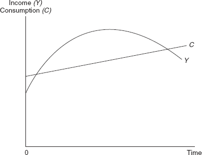
Figure 9.2 Relationship Between Income and Consumption: The Life Cycle Hypothesis
Figure 9.2 depicts the relationship between income and consumption based on the life cycle hypothesis
| where, | x-axis = | time, in say, years |
| y-axis = | income and consumption streams | |
| Curve Y = | a profile of the income stream earned by an individual during his entire life | |
| Curve C = | the consumption stream during his entire life |
The curve Y depicts the income stream of the individual in each year. It starts from the year when the individual begins with full time employment, reaches a maximum when he approaches his middle years and falls thereafter. The curve C, which depicts the consumption stream, curves as an upward sloping line showing consumption level that increases steadily from year to year. If an individual decides not to make any bequests, then he will attempt at making the present value of his income stream equal to the present value of his consumption stream. In simpler terms, it implies that he would spend his entire income on consumption over the entire period of his life.
Figure 9.2 shows that:
- In the initial years of his working life, the individual is a dissaver or in other words a net borrower and thus his consumption curve is above the income curve.
- In the middle years of his working life, the individual is a saver and thus his consumption curve is below the income curve. He may be paying back his earlier debts and also investing his savings in interest-earning assets.
- In the later years of his working life, the individual is once again a dissaver and his consumption curve is above the income curve. However, the difference now is that he finances his dissavings not through borrowing but through the savings that he built up in the earlier years of his life.
From the above analysis, the following are analysed.
- The average propensity to consume will be smaller at higher levels of a family’s income. The families with the higher income levels are, in general, those families whose incomes are high because the income earner in the family is in the middle years of his working life.
- The average propensity to consume will be larger at lower levels of a family’s income. The families with the lower income levels are, in general, those families whose incomes are low because the income earner in the family is in the initial years or in the later years of his working life.
As far as the changes in the income levels are concerned, according to the life cycle hypothesis, any increase or decrease in the income will not have much of an influence on the consumption level as the life cycle consumptions stream have already taken into consideration such expected changes in the income levels. They will be considered as temporary deviations from the expected income in one’s life. However, unexpected changes in the current income levels which have a major impact on the expected income levels will have a considerable effect on the consumption levels. Thus, the theory lays an emphasis on how to maintain a stable standard of living in the face of changes in the lifetime income stream. It views individuals as planning their lifetime consumption stream in the best possible manner. It links consumption and thus savings behaviour to the demographic aspects, like the age distribution of the population.
Criticisms: The hypothesis is based on some assertions which are not correct; some of them are as follows:
- The life cycle hypothesis is based on the assumption that an individual has a clear vision about his future expected income stream or what he expects to earn in his entire lifetime. He is also aware of things like the present and future interest rates and the returns on his investments.
- The individual is expected to have all the information that he requires to plan his life cycle income and consumption streams.
- The analysis is not able to bring about a clear and direct relationship between current consumption and current income.
- The empirical evidence does not support the life cycle hypothesis.
- The life cycle hypothesis maintains that individuals stabilize their consumption levels over a period of time as they relate their consumption streams to the expected lifetime income stream.
- The average propensity to consume will be smaller at higher levels of a family’s income.
- The average propensity to consume will be larger at lower levels of a family’s income.
- Any increase or decrease in the income will not have much of an influence on the consumption level.
OTHER FACTORS INFLUENCING CONSUMPTION
Besides income, there are many other factors that have an affect on the consumption levels. These include:
(1) Rate of interest: Though it is quite certain that the rate of interest influences the allocation of the aggregate disposable income between saving and consumption, it is highly uncertain as to the whether a high rate of interest implies that less of the disposable income will be devoted to consumption and more to saving. Any change in the interest rate may effect saving in either way for an individual’s saving is directly related to the interest rate. An increase in the rate of interest has a two-fold effect:
- Substitution effect: It produces a substitution of present consumption to future consumption. This implies that due to the substitution effect, more will be saved at high interest rates (to be able to consume more in the future).
- Income effect: It increases the individual’s future income as compared to the present income. This may, in fact, encourage him to take a part of this increased future income in the form of increased present consumption. Hence, this implies less saving at high interest rates due to the income effect.
For individuals with high incomes, there is a tendency to save a large part of their incomes. Therefore, the income effect may outweigh the substitution effect. The high rate of interest may lead to a reduction in the current saving. The supply curve showing the relationship between the rate of interest and saving will initially have an upward slope to the right but may bend backwards at some very high rate of interest implying that savings decrease for all higher rates.
For individuals with low incomes, even at high interest rates saving is only a small part of the income. Therefore, the substitution effect may outweigh the income effect. The saving will fluctuate directly with the interest rate. The supply curve showing the relationship between the rates of interest and saving will slope upwards towards the right.
We find that at a high rate of interest while some individuals save more, others save less. However, this is applicable only to those individuals who save. As far as the dissavers are concerned, they finance their current consumption requirements out of their current income. Any excess of current consumption will have to be financed either by borrowing or by drawing from the past saving. High interest rates will discourage them from borrowing and, thus, reduce on dissavings. In other words, this implies that the there is direct relationship between saving and interest rate.
It appears that for some savers, the supply curve showing the relationship between the rates of interest and saving may slope upwards towards the right, depicting a direct relationship with the rate of interest. For the other savers, the supply curve may ultimately bend backwards at some very high rate of interest implying that savings are inversely related to the interest rate. As far as the dissavers are concerned, the supply curve will vary directly with the interest rate. The problem that arises is that the general aggregate supply curve, which is a summation of all these individual supply curves, cannot be specified. A simple relationship between the interest rate and aggregate personal saving (and hence, consumption) cannot be specified under these circumstances.
(2) The price level: To analyse the influence of the price of the consumer goods and services on consumption, it is first important to understand that we are here interested in aggregate consumption expenditures (and not the expenditures on a single good). When there is an increase or a decrease in the price level of the consumer goods, the consumer will react by either spending more or less of his income on goods and services.
It is important to understand that if the current disposable income rises or falls in proportion to the consumer price level, then the real disposable income will not change. If it rises or falls disproportionately, then the real disposal income will also rise or fall accordingly.
Money illusion: Consumers may often be subjected to money illusion. Suppose that during a certain time period the price level increases by 20 per cent and the current disposable income also increases by 20 per cent, there may be some families who realize that their real income is unchanged and thus they do not suffer any money illusion. They increase their current consumption and current saving by 20 percent and, thus, their real consumption and real saving remains unchanged.
However, there may be families of a different kind who may be subject to a money illusion. They are of two kinds which are as follows:
(1) Those families who may consider only the increase in the prices and may fail to notice the increase in their current incomes. These families feel that they are worse off as their real income has reduced. Thus, they react to the situation by cutting down on their saving and increasing their consumption. There is an increase in their real consumption.
(2) Those families who may consider only the increase in their current incomes and may fail to notice the increase in the price level. These families feel that they are better off. They react to the situation by increasing their saving and decreasing their consumption. There is a decrease in their real consumption.
If the consumers are not subject to a money illusion, then:
(1) If the change in the price level is accompanied by a proportionate change in the income, there will be no change in the consumer’s real income. Hence, his real consumption will remain unchanged.
(2) If the change in the price level is accompanied by a disproportionate change in the income, there will be a change in the consumer’s real income. Hence, his real consumption will change. When there is an increase in the price level, there will be a decrease in the real income. Hence, the individual will reduce his real consumption but it is to be noted that the fraction of his real income devoted to consumption may actually increase. When there is a decrease in the price level, there will be an increase in the real income. The individual will increase his real consumption but the fraction of his real income devoted to consumption may actually decrease.
Price expectations: Till now, we have focused on the realized changes in the consumer price level and the effects which follow from it. However, it is possible that real consumption may change due to the mere expectations of a change in the price level.
If the price level has been increasing for some time, then it is possible that the consumers may expect an even higher price level tomorrow. Hence, they may increase their real consumption by spending a large fraction of their real income on consumption.
If the price level has been decreasing for some time, then it is possible that the consumers may expect an even lower price level tomorrow. Hence, they may decrease their real consumption by spending a smaller fraction of their real income on consumption. They prefer to postpone their consumption to the future in which they expect lower prices.
The expectations of a price change are crucial in determining the consumption expenditures of an individual. In fact, consumer expectations can undergo a change even due to social, political and economic changes leading to a change in the consumption.
(4) Income distribution: The distribution of income plays an important role in determining the consumption expenditures. The fraction of the income, which is allocated to consumption, is lower at the higher levels of a family’s income and higher at the lower levels of a family’s income. It follows that the more equal is the income distribution the larger is the fraction of the income that is devoted to consumption. However, it is not necessary that a redistribution of the income in favour of the low income families will increase the fraction of the income that is devoted to consumption. This is due to many reasons; some of them are:
- In the short period, the changes in the distribution of income may be moderate and yearly changes are very insignificant. The government may, to some extent, try to make the income distribution more equal through a progressive tax. But even then, past experience shows that such changes in the income distribution do not bring about much of a change in the consumption expenditures.
- A redistribution of the income will involve additions to the income of some and deductions from the income of the others. It is important to observe that while consumption expenditures from the total income depend on the average propensity to consume, the consumption expenditures from the additions to or deductions from the total income depend on the marginal propensity to consume. Thus, the immediate impact of any additions or reductions will depend on the marginal propensity to consume. But the marginal propensity to consume (as compared to the average propensity to consume) is more or less the same at different levels of a family’s income. Thus, it seems that a redistribution of the income does not lead to much of an increase in the fraction of the income devoted to consumption.
(5) Financial assets: The volume of the financial assets accumulated by the individual is also important in determining his consumption expenditures. These assets may include cash, demand and time deposits, saving deposits, stocks and bonds. A family, which has amassed larger amounts of such assets, will spend more on consumption as it does not feel any need to add to its already large accumulation of the financial assets. Hence, it will devote a smaller fraction of its income to saving and a larger one to consumption. On the other hand, a family with a smaller accumulation of the financial assets will devote a larger fraction of its income to saving and a smaller one to consumption.
The above analysis is subject to some qualifications; these are:
(1) The increase in the consumption will depend on the ownership of the financial assets. If the increase in the financial assets is concentrated among the upper class, the consumption may not increase much because the rich save a large part of their income.
(2) For many families, the acquisition of a few financial assets may simply stimulate their appetite for more of these assets. Hence, they may cut down on consumption in favour of savings which will facilitate them to acquire more financial assets.
Though these assets are one of the most important non-income factors, which influence consumption but evidence seems to support the view that these assets do not have a major influence on the consumption expenditures.
RECAP
- The other factors, which influence consumption, do play an important role but the income level continues to be the most important factor that influences consumption.
SUMMARY
INTRODUCTION
The present chapter analyses the relationship between consumption and income by looking at four hypotheses—absolute income hypothesis, relative income hypothesis, permanent income hypothesis and the life cycle hypothesis.
ABSOLUTE INCOME HYPOTHESIS
- The basic principle of absolute income hypothesis is that the individual consumer will determine the fraction of his current income that he will allocate to consumption on the basis of his absolute income level.
- Everything else remaining unchanged, an increase in the income will lead to a decrease in the fraction of the income allocated to consumption.
- Families with low incomes have a high marginal propensity to consume as they spend a large proportion of their incomes on consumption where as families with high incomes have a low marginal propensity to consume as they spend a small proportion of their incomes on consumption.
- For the average family, there is a decrease in the average propensity to consume when it climbs up the income scale.
RELATIVE INCOME HYPOTHESIS
- According to the relative income hypothesis, the fraction of a family’s income that will be allocated to consumption will depend on its income level relative to the income level of the other families with which it classifies itself.
- If a family’s absolute income increases but its relative income (income relative to the other families with which it classifies itself) remains unchanged, then its distribution of income between consumption and savings will also remain unchanged.
- If a family’s income remains the same but its relative income (income relative to the other families with which it classifies itself) deteriorates because there occurs an increase in the income of the other families with which it classifies itself, then there will be a change in the family’s distribution of income between consumption and savings.
- The ‘relative income hypothesis’ lays emphasis on the emulative nature of a family and on what Duesenberry called the ‘demonstration effect’.
PERMANENT INCOME HYPOTHESIS
- The permanent income hypothesis puts forward the view that consumption is related to the permanent income.
- The average propensity to consume expressed in terms of the permanent income is the same on an average for all families whether rich or poor.
- Friedman has split up the measured income into two components, the permanent income and the transitory income. His main argument is that the permanent consumption depends on the permanent income.
- Another argument put forward by Friedman here is that transitory consumption is not related, in any way, to transitory income. This implies that any unanticipated increases or decreases in the income level lead to comparable increases or decreases in the saving (and not in consumption).
LIFE CYCLE HYPOTHESIS
- The life cycle hypothesis puts forward the view that consumption is related to the present value of the individual’s income or wealth.
- It argues that consumption is related to the present value of the individual’s income or wealth. This suggests that the individual sustains a constant or slightly increasing level of consumption over his entire life cycle.
- The average propensity to consume will be smaller at higher levels of a family’s income.
- The average propensity to consume will be larger at lower levels of a family’s income.
- As far as the changes in the income levels are concerned, according to the life cycle hypothesis, any increase or decrease in the income will not have much of an influence on the consumption level.
OTHER FACTORS INFLUENCING CONSUMPTION
- Besides income, there are many other factors like the rate of interest, price level, price expectations, income distribution and financial assets, which influence the consumption levels.
- Rate of interest: It is highly uncertain whether a high rate of interest implies that less of the disposable income will be devoted to consumption and more to saving.
- The price level: When there is an increase or a decrease in the price level of the consumer goods, the consumer will react by either spending more or less of his income on goods and services. Consumers may often be subject to money illusion.
- Price expectations: It is possible that real consumption may change due to the mere expectations of a change in the price level. If the price level has been increasing for some time, then it is possible that the consumers may expect an even higher price level tomorrow. Hence, they may increase their real consumption by spending a large fraction of their real income on consumption.
- Income distribution: The distribution of income plays an important role in determining the consumption expenditures. The fraction of the income, which is allocated to consumption, is lower at the higher levels of a family’s income and higher at the lower levels of a family’s income. It follows that the more equal is the income distribution the larger is the fraction of the income that is devoted to consumption. It seems that a redistribution of the income does not lead to much of an increase in the fraction of the income devoted to consumption.
- Financial assets: The volume of the financial assets accumulated by the individual is also important in determining his consumption expenditures. These assets may include cash, demand and time deposits, saving deposits, stocks and bonds. A family, which has amassed larger amounts of such assets, will spend more on consumption as it does not feel any need to add to its already large accumulation of the financial assets.
REVIEW QUESTIONS
TRUE OR FALSE QUESTIONS
- According to the absolute income hypothesis, everything else remaining unchanged, an increase in the income will lead to a decrease in the fraction of the income allocated to consumption.
- Families with high incomes have a high marginal propensity to consume as they spend a large proportion of their incomes on consumption.
- The high income families save a large proportion of their incomes as compared to the low income families.
- The permanent income hypothesis puts forward the view that consumption is related to the relative income.
- The ‘relative income hypothesis’ lays emphasis on what Duesenberry called the ‘demonstration effect’.
VERY SHORT-ANSWER QUESTIONS
- Why do families with high incomes have a low marginal propensity to consume?
- Give a brief criticism of Keynes’ absolute income hypothesis.
- According to the life cycle hypothesis, the average propensity to consume will be smaller at higher levels of a family’s income and larger at lower levels of a family’s income. Why?
- What is money illusion? How does it affect consumption?
- How do price expectations influence consumption? Discuss.
SHORT-ANSWER QUESTIONS
- What is Duesenberry’s ‘demonstration effect’? Explain.
- What is the permanent income according to Friedman?
- What are permanent consumption and transitory consumption? How are they related to the permanent income and transitory income? Explain.
- What is the relationship between income and consumption according to the life cycle hypothesis? Explain.
- Analyse the effects of income distribution and a change in the holding of financial assets on consumption.
LONG-ANSWER QUESTIONS
- ‘The basic principle of absolute income hypothesis is that the individual consumer will determine the fraction of his current income that he will allocate to consumption on the basis of his absolute income level.’ Comment.
- Depict the relationship between income and consumption in the absolute income hypothesis with the help of a diagram.
- ‘According to the relative income hypothesis, the fraction of a family’s income that will be allocated to consumption will depend on its income level relative to the income level of the other families with which it classifies itself.’ Comment.
- What is the permanent income hypothesis? Explain.
- ‘The life cycle hypothesis puts forward the view that consumption is related to the present value of the individual’s income or wealth.’ Is this correct? Comment.
TRUE OR FALSE QUESTIONS
- True. The basic principle of the absolute income hypothesis is that the individual consumer will determine the fraction of his current income that he will allocate to consumption on the basis of his absolute income level. Everything else remaining unchanged, an increase in the income will lead to a decrease in the fraction of the income allocated to consumption.
- False. Families with low incomes have a high marginal propensity to consume as they spend a large proportion of their incomes on consumption.
- True. The high income families save a large proportion of their incomes as compared to the low income families as they are left with a large proportion of their incomes after fulfilling their consumption needs.
- False. The permanent income hypothesis puts forward the view that consumption is related to the permanent income.
- True. The ‘relative income hypothesis’ lays emphasis on the emulative nature of a family and on what Duesenberry called the ‘demonstration effect’ where families are influenced by the other family’s standard of living and thus try to ‘keep up with the Joneses’.