17
The IS–LM Framework for a Three Sector Model
After studying this topic, you should be able to understand
- In a three sector model, two new variables are included: government expenditure and taxation, G and T.
- There is only one combination of income and the interest rate at which there exists simultaneous equilibrium in the goods and money market.
- An increase in government expenditure by ΔG shifts the IS curve to the right by an amount equal to 1/1 – b × ΔG.
- The impact of taxes is felt through a change in the consumption level.
- A change in the money supply disturbs the money–market equilibrium causing a shift in the LM curve.
- By how much does the national income change in response to the monetary and fiscal policies depends on the elasticities of the IS and the LM curves.
- An expansionary fiscal policy shifts the IS curve to the right and leads to an increase in both the income level and the interest rate.
- An expansionary monetary policy shifts the LM curve to the right and leads to an increase in the income level but a decrease in the interest rate.
INTRODUCTION
This chapter is an extension of Chapter 16 which extends the IS–LM two sector model to a three sector model where there exists the government sector in addition to the households and the firms. The shifts in the IS curve due to the changes in fiscal policy and the shifts in the LM curve due to changes in monetary policy are also analysed.
The chapter goes on to discuss the effectiveness of monetary and fiscal policies in the different ranges of the LM curve. (Refer to Appendix B for the IS–LM framework for a four sector model)
THE IS–LM MODEL FOR A THREE SECTOR ECONOMY
The construction of a three sector model involves the inclusion of two new variables which pertain to the government sector, government expenditure and taxation. The analysis is based on certain assumptions:
- The price level is constant.
- At that constant price level, the firms are willing to supply whatever output is demanded.
- The short-run aggregate supply curve is perfectly elastic till the full employment level of output.
- Government expenditure is autonomous; hence, G =
 .
. - Taxes are a linear function of income. Thus, T =
 + tY where is the autonomous tax (which is independent of the income level) while t is the income tax rate.
The IS–LM model emerged as an aftermath of the Keynesian revolution. It showed how the economists from the period of the 1940s to the 1960s regarded the Keynesian economics and the classical economics. Later, many other macroeconomic models also came up like the Harrod–Domar growth model and the multiplier–accelerator business-cycle model. However, these failed to gain as much popularity as some of the other models like the IS–LM model.
THE GOODS MARKET EQUILIBRIUM IN A THREE SECTOR ECONOMY: THE IS CURVE
As already observed, there are two approaches to determine the equilibrium level of income. In a three sector economy, they can be expressed as
(1) Aggregate Demand–Aggregate Supply Approach
Aggregate demand = Total value of output (or income)
or
Y = C + I + G
(2) Injections equal Leakages Approach
I + G = S + T
We have consumption function as C = C(Y); investment function as I = I(r); government expenditure G = ![]() ; saving function as S = S(Y); tax as T =
; saving function as S = S(Y); tax as T = ![]() + tY and equilibrium condition as Y = C(Y) + I(r) +
+ tY and equilibrium condition as Y = C(Y) + I(r) + ![]() .
.
The two equilibrium conditions can be used to develop a graphical approach to the derivation of the IS curve as in Figure 17.1.
In Figure 17.1 starting with a two sector model, Quadrant A shows the investment curve, I. Corresponding to the saving function S1 in Quadrant C, the two sector goods market equilibrium is represented by the curve IS1 in Quadrant D. The investment curve, I of Quadrant A and the savings curve, S1 of Quadrant C yields the curve ISl in Quadrant D. Quadrant D shows the goods market equilibrium in a three sector economy where the IS curve depicts the different combinations of the interest rates and the output levels at which planned investment equals saving or planned spending is equal to the income.
Next assume the government sector is introduced in the model or, in other words, we have a three sector model. In Quadrant A, government expenditures have been added to the investment curve to get the I + G curve. As government expenditures are independent of the interest rate, I + G curve lies to the right of the investment curve as shown in the figure.
Quadrant B gives the injections leakages equality in the form of a 45 degree line drawn through the origin. At all points along this 45 degree line, injections equal leakages or I + G = S + T.
Quadrant C shows the saving function S. When a tax is imposed, the saving curve will shift to the right by the amount of the tax to get the adjusted saving curve S2. When taxes are added to the adjusted saving function, we get the S2 + T curve in Quadrant C of Figure 17.1.
The investment curve I of Quadrant A and the saving curve S of Quadrant C yielded the curve IS1 in Quadrant D. The investment plus government expenditure curve (I + G) of Quadrant A and the saving plus tax curve (S2 + T) of Quadrant C yields the curve IS2 in Quadrant D.
THE MONEY–MARKET EQUILIBRIUM IN A THREE SECTOR ECONOMY: THE LM CURVE
In a three sector economy, the analysis of the money market will remain the same as in the two sector economy as government expenditure and taxes do not influence either the demand for money or the supply of money.

Figure 17.1 The Goods Market Equilibrium in a Three Sector Economy: The IS Curve
Equilibrium in the Two Markets: The Goods Market and Money Market
The IS Curve: An Algebraic Explanation
The goods market is in equilibrium when
Aggregate demand = Total value of output (or income)
or
Y = C + I + G
But,
C = Ca+b Yd,
G = ![]() ,
,
Yd = Y – T,
T = ![]() + tY
+ tY
Thus,
Y = Ca + bYd + ![]() – hr +
– hr + ![]()
Y = Ca + b(Y – T) + ![]() – hr +
– hr + ![]()
Y = Ca + b[Y – (![]() + tY)] +
+ tY)] + ![]() – hr +
– hr + ![]()
Y = Ca + bY – b![]() – btY +
– btY + ![]() – hr
– hr ![]()
Y – bY + btY = Ca – b![]() +
+ ![]() – hr +
– hr + ![]()
Y(1 – b + bt) = Ca – b![]() +
+ ![]() – hr +
– hr + ![]()
Equation (1) represents the IS curve in a three sector economy.
Numerical Illustration 1
Suppose the consumption and investment functions are as follows:
C = 10 + 0.5Y
I = 80 – 8r.
- Find the equation of the IS curve.
- Suppose the government sector is introduced in the model. Now C = 10 + 0.5 Yd (where Yd = Y – T), I = 80 – 8r, G = Rs. 20 crores and T = Rs. 30 crores. Find the equation of the IS curve.
Solution
- Equation of the IS curve
Y = C + I
Y = 10 + 0.5Y + 80 – 8r
0.5Y = 90 – 8r
Y = 180 – 16r
- Equation of the IS curve when the government sector is introduced in the model:
Y = C + I + G
Y = 10 + 0.5 (Y – 30) + 80 – 8r + 20
0.5Y = 90 – 8r – 15 + 20
0.5Y = 95 – 8r
Y = 190 – 16r
The LM Curve: An Algebraic Explanation
The money–market equilibrium is similar to that of a two sector economy.
Thus,
md = ms
But,
md = mt + msp
| where, | md = total demand for money |
| mt = kY (transactions demand for money) | |
| msp = g(r) (speculative demand for money) |
We assume that the speculative demand for money is a linear function (rather than a curve). Hence, we have msp = ![]() sp – g(r).
sp – g(r).
From the above, we have Supply of money ms = ![]() a
a
Demand for money md = kY + ![]() sp – g(r)
sp – g(r)
The money–market equilibrium condition can be written as
Thus,
Equation (2) represents the LM curve.
RECAP
- With the inclusion of the two new variables, G and T, the IS curve represents the goods market equilibrium whereas the LM curve represents the money–market equilibrium.
EQUILIBRIUM IN THE GOODS AND THE MONEY MARKET IN A THREE SECTOR ECONOMY
We have already observed in Chapter 16 that there is only one combination of income and the rate of interest at which both the goods and the money market are in equilibrium. This has been depicted in Figure 17.2. This combination exists at point E at which the IS and LM curves intersect to determine the equilibrium rate of interest at r* and the equilibrium level of income at Y*. It is important to note that at all other points, there exists disequilibrium in either the goods market or the money market.
All combinations of income and interest that lie above and towards the right of the IS curve, like point R, indicate a situation where Y > C + I + G or saving plus taxes is greater than planned investment plus government expenditures. There exists an excess supply of goods. Hence, the level of income will fall.
BOX 17.2
The initial IS–LM model (as compared to the new IS–LM model) plays an important role in policy decisions. However, it is being subject to criticism in that it is an obsolete instrument of monetary policy. It is unable to explain the existence of a high inflation rate and high unemployment rate simultaneously in the economy. However, attempts are being made to revive the initial IS–LM model through the expectation concepts.
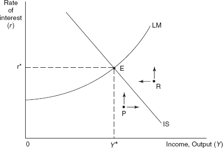
Figure 17.2 Equilibrium in the Goods and the Money Market in a Three Sector Economy
All combinations of income and interest that lie below and towards the left of the IS curve, like point P, indicate a situation where Y < C + I + G or saving plus taxes is less than planned investment plus government expenditures. There exists an excess demand for goods. Thus, there will be an increase in the income level.
Similarly as far as the LM curve is concerned, at all combinations of income and interest that lie below and towards the right of the LM curve, like point R, the demand for money is greater than the supply of money or there is an excess demand for money. Hence, the rate of interest will rise.
At all combinations of income and interest that lie above and towards the left of the LM curve, the demand for money is less than the supply of money or there is an excess supply of money. Hence, the rate of interest will fall.
It is only at point E that there is equilibrium in both the goods and money markets which will remain unchanged until a shift in the IS or LM curve disturbs the equilibrium.
RECAP
- The point of equilibrium will remain unchanged until it is disturbed by a shift in the IS or LM curve.
Numerical Illustration 2
Suppose the consumption and investment functions are as follows:
C = 60 + 0.60Yd(where Y = Yd – T)
I = 150 – 8r
Also, the government expenditure and taxes are
G = Rs. 50 crores
T = Rs. 50 crores
Assume that the supply of money is Rs. 120 crores. The demand for money function is md = 0.25 Y – 5r.
Find
- the equation of the IS curve.
- the equation of the LM curve.
- the simultaneous equilibrium for the IS curve and LM curves and plot it.
- IS equation:
Y = C + I
Y = 60 + 0.60(Y – 50) + 150 – 8r + 50
Y = 230 + 0.60Y – 8r
0.40Y = 230 – 8r
Y = 575 – 20r
- LM equation:
md = 0.25Y – 5r
ms = 120
In equilibrium,
md = ms
Thus,
0.25Y – 5r = 120
0.25Y = 120 + 5r
Y = 480 + 20r
- Simultaneous equilibrium for the IS curve and LM curves
IS = LM
575 – 20r = 480 + 20r
40r = 95
r = 2.375%
Y = 575 – 20 × 2.375
Y = 527.5
Simultaneous equilibrium for the IS curve and LM curves exists when Y = 527.5 and r = 2.375%.
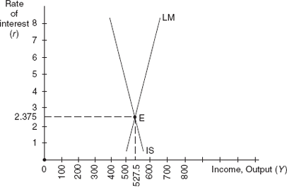
Figure 17.3 Simultaneous Equilibrium for IS and LM Curves Exist When Y = 527.5 and r = 2.375%
SHIFTS IN THE IS CURVE DUE TO CHANGES IN FISCAL POLICY
In Chapter 16 we had observed that a shift in either the investment function or the consumption function leads to a shift in the IS curve. Similarly, the effects of a change in the fiscal policy can be analysed in terms of its influence on the IS curve and the resulting changes in income and the rate of interest. It is to be remembered that a fiscal policy relates to the government expenditures and its taxes.
A Change in Government Expenditure
In Figure 17.4, the initial equilibrium is at point E1 determined by the intersection of the IS1 and LM curves with the equilibrium income and the rate of interest at Y1 and r1 respectively.
An increase in government expenditure by ΔG shifts the IS curve to the right by an amount equal to the government expenditure multiplier times the change in government expenditure, 1/1 – b × ΔG. (We had discussed in Chapter 7 that the government expenditure multiplier is GM = ΔY/ΔG = 1/1 – b). Thus, the new IS curve is IS2 with the equilibrium at point E2. The equilibrium income and the rate of interest are Y2 and r2, respectively.
The above analysis shows that an increase in government expenditure brings about an increase in income from Y1 to Y2 and an increase in the rate of interest from r1 to r2.
One would expect that the increase in the government expenditure would result in an increase in the income level by an amount equal to the multiplier times the increase in the government expenditure or, in other words, by an amount equal to 1/1 – b × ΔG. In that case, equilibrium would be at point E′ on the IS2 curve and the increase in income would be from Y1 to Y′. Instead, the equilibrium is at E2 while the increase in income is from Y1 to Y2 only. This is due to the crowding out effect.
Crowding Out
The level of government expenditure, G, is an important component of aggregate demand. As already discussed, Figure 17.4 analyses the effects of a shift in the IS curve due to an increase in aggregate demand. The initial equilibrium is at point E1. Given the rate of interest at r1, there is an increase in government expenditure and thus in the aggregate demand. To meet the increased demand, there will be an increase in the level of output. The IS curve will shift from IS1 to IS2 and equilibrium will move from point E1 to point E′ at the rate of interest, r1 There will be an increase in the equilibrium income from Y1 to Y′.
Crowding out is a situation which arises when an expansionary fiscal policy–for example, an increase in government expenditure–leads to an increase in the rate of interest, thus leading to a decrease in private investment.
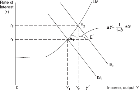
Figure 17.4 Shift in the IS Curve Due to Changes in Fiscal Policy
At E′ though there exists goods market equilibrium, there is disequilibrium in the money market. This is because the increase in the income has generated an excess demand for money. Therefore, there will occur an increase in the rate of interest leading to a decrease in investment and hence in the aggregate demand. After all the adjustments for the increase in the government expenditures and the dampening effects of the higher rate of interest on investment are taken into consideration, both the goods and the money market are simultaneously in equilibrium only at point E2. It is only at this point that the planned spending equals income and the demand for money equals the supply of money. Thus, an increase in government expenditure (fiscal expansion) does lead to an increase in the income level, but it is to be noted that the increase in the rate of interest has a dampening effect on the expansion. In Figure 17.4, a comparison between the equilibrium at E2 and E′ in the goods market shows that the increase in the government expenditure leads to an increase in the income level from Y1 to Y2 (and not Y′).
Crowding out is a situation which arises when an expansionary fiscal policy–for example, an increase in government expenditure–leads to an increase in the rate of interest, thus leading to a decrease in private investment. Hence, the adjustments which occur in the rate of interest have a dampening effect on the increase in the output.
We consider two cases:
- In an economy with the level of output at the full employment level, an increase in government expenditures will cause an increase in aggregate demand and, hence, an increase in the rate of interest. This will continue till the initial increase in the aggregate demand is totally crowded out.
- In an economy with the level of output below the full employment level, whenever there is an increase in government expenditures firms will hire more workers to increase the level of output. Hence, there occurs an increase in both the interest rate and the income level. In such a situation, there will not be a full crowding out.
A Change in Taxes
The impact of taxes is felt through a change in the consumption level. In Figures. 17.5 and 17.6, which show the impact of a tax, the economy’s initial equilibrium is at point E1 determined by the intersection of the IS1 and LM curves with the equilibrium income and the rate of interest at Y1 and r1, respectively.
Figure 17.5 depicts the impact of an increase in taxes. Suppose the government increases the tax by ΔT (there is no change in government expenditures), this will shift the IS curve to the left by an amount equal to the tax multiplier times the change in the tax, b/1 – b × ΔT. (We had observed in Chapter 7 that the tax multiplier is GT = ΔY/ΔT = b/1 – b). Thus, the new IS curve is IS2 with the equilibrium at point E2. The equilibrium income and the rate of interest are Y2 and r2, respectively. Thus, an increase in tax brings about a decrease in income from Y1 to Y2 and a decrease in the rate of interest from r1 to r2.
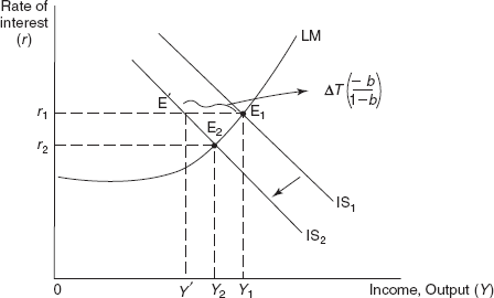
Figure 17.5 Shift in the IS Curve Due to an Increase in Tax
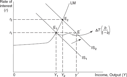
Figure 17.6 Shift in the IS Curve Due to a Decrease in Tax
One would expect that an increase in the tax would result in a decrease in the income level by an amount equal to the tax multiplier times the increase in the tax, or in words b/1 – b × ΔT. In that case, the new equilibrium would be at point E′ on the IS2 curve and the decrease in income from Y1 to Y′. Instead, the equilibrium is at E2 while the decrease in income is from Y1 to Y2 only. The reason for this is that an increase in the tax results in a decrease in the consumption level which leads to a decrease in the production of the goods and services causing a decrease in the income levels. Hence, individuals demand less money leading to decrease in the interest rates. The decrease in the interest rates is responsible for an increase in investment, thus, offsetting the decrease in the consumption levels to some extent. The Keynesian model had ignored these effects and, thus, exaggerated the effects of an increase in the taxes.
Figure 17.6 depicts the impact of a decrease in taxes. Suppose that the government decreases the tax by ΔT (there is no change in government expenditures). This will lead to a shift in the IS curve to the right by an amount equal to the tax multiplier times the change in the tax, b/1 – b × ΔT. The new IS curve is IS with the equilibrium at point E2. The equilibrium income and the rate of interest are Y2 and r2, respectively. Thus, a decrease in tax brings about an increase in the income from Y1 to Y2 and an increase in the rate of interest from r1 to r2.
One would expect that a decrease in the taxes would result in an increase in the income level by an amount equal to the tax multiplier times the decrease in the taxes, or in words b/1 – b × ΔT. Then, the new equilibrium would be at point E′ on the IS2 curve and the increase in income from Y1 to Y′. Instead, the equilibrium point is E2 while the increase in income from Y1 to Y2 only. The reason for this is that a decrease in the taxes results in an increase in the consumption level which leads to an increase in the production of the goods and services causing an increase in the income levels. Hence, individuals demand more money leading to an increase in the interest rates. The increase in the interest rates is responsible for the firms reducing their investments. The Keynesian model had ignored these effects and understated the effects of a decrease in the taxes.
RECAP
- The increase in the income due to the increase in the government expenditure should be equal to 1/1 –b × ΔG.
- Due to the crowding out effect, the increase in income is much smaller than 1/1 – b × ΔG.
- As far as the impact of an increase in tax is concerned, the decrease in the interest rates is responsible for an increase in investment, thus, offsetting the decrease in the consumption levels to some extent.
- As far as the impact of a decrease in tax is concerned, the increase in the interest rates is responsible for a decrease in investment, thus, offsetting the increase in the consumption levels to some extent.
SHIFTS IN THE LM CURVE DUE TO MONETARY POLICY
The monetary policy operates through the changes in the supply of money. A change in the money supply disturbs the money–market equilibrium causing a shift in the LM curve. The shift in the LM curve influences the income level and the rate of interest.
Let us examine the effects of an increase in the money supply. In Figure 17.7, the initial equilibrium is at point E1 determined by the intersection of the curves IS and LM1. The equilibrium income is Y1 while the equilibrium rate of interest is r1.
The mechanism by which the changes in the monetary policy affect the aggregate demand and, thus, the income level is called the monetary transmission process.
Suppose there is an increase in the money supply. Thus at the prevailing rate of interest r1, individuals are now holding excess money in their portfolio which they will try to deposit in the banks, buy bonds, etc. Hence, there will be a decrease in the interest rates. The equilibrium moves to point E′ at which there is equilibrium in the money market and the individuals are willing to hold a larger quantity of money due to a decrease in the interest rate. However, at point E′ there is disequilibrium in the goods market. The decrease in the interest rate will encourage investment leading to an increase in the income level. As a result, there occurs a movement up the LM2 until a new equilibrium is established at point E2, determined by the intersection of the curves IS and LM2. The equilibrium income increases to Y2 while the equilibrium rate of interest falls to r2.
The mechanism by which the changes in the monetary policy affect the aggregate demand and, thus, the income level is called the monetary transmission process.
RECAP
- A shift in the LM curve affects the income level and the rate of interest.
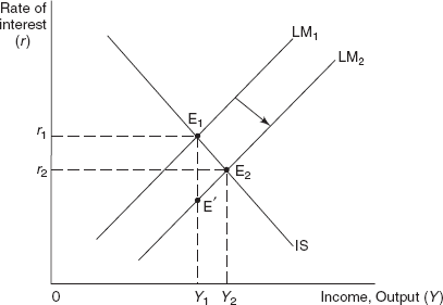
Figure 17.7 The Effects of an Increase in the Money Supply
THE ELASTICITIES OF IS AND LM CURVES AND THE EFFECTIVENESS OF MONETARY AND FISCAL POLICIES
We have observed the impact of the monetary and fiscal policies in bringing about changes in the national income. However, we have yet to determine by how much the national income will change in response to the policies. This responsiveness depends on the elasticities of the IS and the LM curves.
The Elasticities of IS and LM Curves
The Elasticity of LM Curve: Given the supply of money in an economy, the LM curve has a positive slope as in Figure 17.8. For most analytical purposes, it can be divided into three ranges:
- Keynesian range: At some very low rate of interest, say r1 speculative demand for money becomes perfectly elastic or infinity. At this rate of interest, all expect the interest rate to increase in the future and, thus, become bears. Hence, all individuals prefer to hold only cash and no one prefers to hold bonds. In this range, no amount of monetary expansion can lower the interest rate. The extra liquidity, which has been created by the monetary authorities, is trapped in the asset portfolio of the public. This range is also called the liquidity trap. The rate of interest serves as the minimum and cannot fall any further. In this range, the LM curve is horizontal and the interest elasticity is infinity.
- Classical range: At some very high rate of interest, the speculative demand for money becomes perfectly inelastic. All expect the interest rate to fall in the future and become bulls. Thus, everyone prefers to hold only bonds and no one likes to hold cash. The speculative demand for money becomes zero. In this range, the LM curve is vertical. This is called the classical range as it is in accordance with the classical theory of money where money is demanded for conducting transactions. In this range, the LM curve is vertical and the interest elasticity is zero.
- Intermediate range: This is the range in between the Keynesian range and the classical range. Here, both the transactions and speculative demand for money exist. The interest elasticity in this range is greater than zero.
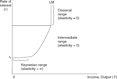
Figure 17.8 The LM Curve
The Elasticity of IS Curve: The IS curve has a positive slope. As far as the elasticity of the IS curve is concerned, it depends on the responsiveness of investment to changes in the interest rate and on the magnitude of the multiplier.
- If investment is insensitive (or independent) to the rate of interest, then the investment curve will be perfectly inelastic. The IS curve will be vertical or perfectly inelastic.
- If investment is sensitive to the interest rate, or in other words it is interest elastic, then the investment curve will be elastic. In that case the IS curve will be elastic; the elasticity being higher, the lower is the marginal propensity to save. (A lower marginal propensity to save implies a higher multiplier.)
Effectiveness of Monetary and Fiscal Policies
The effectiveness of a policy in achieving the economic objectives depends on the elasticity of the IS and LM curves. It is important to note that an expansionary fiscal policy, as it shifts the IS curve to the right, leads to an increase in both the income level and the interest rate. On the other hand, an expansionary monetary policy, as it shifts the LM curve to the right, leads to an increase the income level but a decrease in the interest rate.
Effectiveness of Fiscal Policy
Fiscal Policy relates to the utilization of government expenditure and taxation to achieve some well-defined objectives relating to growth, employment and many others. The fiscal policy has an immediate impact on the goods market and, thus, leads to shift in the IS curve.
In Figure 17.9, we examine the effectiveness of the fiscal policy in the three different ranges of the LM curve:
- Keynesian range or the liquidity trap: Here, fiscal policy is very effective. Initially, the equilibrium exists at the intersection of the IS1 and LM curves to determine the equilibrium income at Y1 and the rate of interest at r1. A fiscal expansion, say an increase in the government expenditure, leads to a shift of the IS1 curve to IS1′. It is important to note that in the range of the liquidity trap, an increase in the government expenditure does not affect the rate of interest and, thus, the level of investment. Hence, there is a full multiplier effect of the increase in the government spending and no dampening effects occur. The income level increases from Y1 to Y1′ while the rate of interest remains unchanged at r1. Hence, fiscal policy is completely effective in the Keynesian range.
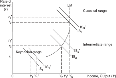
Figure 17.9 Effectiveness of Fiscal Policy
- Classical range: Here, fiscal policy is not effective. Initially, the equilibrium exists at the intersection of the IS3 and LM curves to determine the equilibrium income at Y3 and the rate of interest at r3. A fiscal expansion, say an increase in the government expenditure, leads to a shift of the IS3 curve to IS3′. The income level remains unchanged at Y3 while the rate of interest increases from r3 to r3′.
An increase in government expenditure and the interest rate and an unchanged income level imply that there occurs an offsetting decrease or crowding out of private investment which equals the increase in the government expenditure. Hence, there is full crowding out. Hence, fiscal policy is completely ineffective in the classical range.
- Intermediate range: Here, fiscal policy is effective but it is not as effective as in the Keynesian range. Initially, equilibrium exists at the intersection of the IS2 and LM curves to determine the equilibrium income at Y2 and the rate of interest at r2. A fiscal expansion, say an increase in the government expenditure, leads to a shift of the IS2 curve to IS2′. Thus, the income level increases from Y2 to Y2′ while the rate of interest increases from r2 to r2′.
In this range, the expansionary effect of the fiscal policy does succeed in raising the income level. However, the increase in the income is not as much as in the Keynesian range. This is due to the increase in the interest rate because of which investment decreases and, thus, the expansionary effect of the fiscal policy gets negated to some extent. Thus, fiscal policy is less effective in the intermediate range as compared to the Keynesian range.
Effectiveness of Monetary Policy
Monetary policy relates to changes in the supply of money by the central bank to achieve the objectives relating to growth, employment and others. Monetary policy has an immediate impact on the money market and leads to a shift in the LM curve.
In Figure 17.10, we examine the effectiveness of the monetary policy in the three different ranges of the LM curve with the help of two types of IS curves, one elastic and the other inelastic.
- Keynesian range: Here, monetary policy is completely ineffective.
- Elastic IS curve, IS1: Initial equilibrium exists at the intersection of the IS1 and LM1 curves to determine the equilibrium income at Y1 and the rate of interest at r1. In this range a monetary expansion, a shift in the LM curve from LM1 to LM2, does not lead to an increase in the income level or any changes in the interest rate, which remain at Y1 and r1 respectively. All increases in the supply of money are held as speculative balances and no part of any increases in the money supply are diverted for transactions. Hence, there is no increase in the income level. Hence, monetary policy is completely ineffective in the Keynesian range.
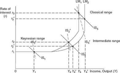
Figure 17.10 Effectiveness of Monetary Policy
- Relatively inelastic IS curve, IS′: As compared to IS1, the curve IS1′ is relatively less elastic. However as with IS1, IS1′ yields the same equilibrium income at Y1 and the rate of interest at r1. The effects of a monetary expansion are also similar.
Monetary policy is ineffective in the liquidity trap whatever the elasticity of the IS curve.
- Elastic IS curve, IS1: Initial equilibrium exists at the intersection of the IS1 and LM1 curves to determine the equilibrium income at Y1 and the rate of interest at r1. In this range a monetary expansion, a shift in the LM curve from LM1 to LM2, does not lead to an increase in the income level or any changes in the interest rate, which remain at Y1 and r1 respectively. All increases in the supply of money are held as speculative balances and no part of any increases in the money supply are diverted for transactions. Hence, there is no increase in the income level. Hence, monetary policy is completely ineffective in the Keynesian range.
- Classical range: Here, monetary policy is completely effective.
- Elastic IS curve, IS3: Initially, equilibrium exists at the intersection of the IS3 and LM1 curves to determine the equilibrium income at Y3 and the rate of interest at r3. A monetary expansion leads to a shift of the LM1 curve to LM2. The income level increases from Y3 to Y3′ while the rate of interest decreases from r3 to r3′.
In the classical range, the speculative demand for money is zero due to the high interest rates. Money is demanded only for transaction purposes. In such a situation, a monetary expansion will push down the rate of interest and, thus, encourage investment leading to an increase in the income level. Monetary policy is totally effective in the classical range in bringing about an increase in the income level.
- Relatively inelastic IS curve, IS3′: As compared to IS3, the curve IS3′ is relatively less elastic. Similar to IS3, IS3′ also yields the same equilibrium income at Y3 and the rate of interest at r3. But as far as the effects of a monetary expansion are concerned, the increase in the income will be lower while the decrease in the interest rate will be much larger than for the elastic IS curve. Monetary policy is completely effective in the classical range whatever the elasticity of the IS curve.
- Elastic IS curve, IS3: Initially, equilibrium exists at the intersection of the IS3 and LM1 curves to determine the equilibrium income at Y3 and the rate of interest at r3. A monetary expansion leads to a shift of the LM1 curve to LM2. The income level increases from Y3 to Y3′ while the rate of interest decreases from r3 to r3′.
- Intermediate range: We had observed that in the Keynesian range, monetary policy is completely ineffective as the entire increase in the money supply is absorbed as speculative money balances. In contrast, in the classical range monetary policy is completely effective as the entire increase in the money supply is absorbed as transactions money balances.
As far as the intermediate range is concerned, monetary policy is effective but not as much as in the classical range because the increase in the money supply is absorbed partly as transactions money balances and partly as speculative money balances.
- Elastic IS curve, IS2: Initially, equilibrium exists at the intersection of the IS2 and LM1 curves to determine the equilibrium income at Y2 and the rate of interest at r2. A monetary expansion leads to a shift of the LM curve to LM2. The income level increases from Y2 to Y2′ while the rate of interest decreases from r2 to r2′.
In the intermediate range, a monetary expansion will push down the rate of interest to some extent and, thus, encourage investment but the increase in the investment in not as much as in the classical range. Hence though there is an increase in the income level, it is not as much as the increase in the classical range.
- Relatively inelastic IS curve, IS2′: In comparison to IS2, the curve IS2′ is relatively less elastic. Similar to IS2, IS2′ also yields the same equilibrium income at Y2 and the rate of interest at r2. Regarding the effects of a monetary expansion, the increase in the income will be smaller than in the case of the elastic IS curve.
Monetary policy is less effective in the intermediate range as compared to the classical range. Thus we find that the fiscal policy is completely effective in the Keynesian range, less effective in the intermediate range and completely ineffective in the classical range. On the other hand, monetary policy is completely ineffective in the Keynesian range, less effective in the intermediate range and completely effective in the classical range.
- Elastic IS curve, IS2: Initially, equilibrium exists at the intersection of the IS2 and LM1 curves to determine the equilibrium income at Y2 and the rate of interest at r2. A monetary expansion leads to a shift of the LM curve to LM2. The income level increases from Y2 to Y2′ while the rate of interest decreases from r2 to r2′.
- Fiscal policy is most effective in the Keynesian range and ineffective in the classical range.
- Monetary policy is most effective in the classical range and ineffective in the Keynesian range.
SUMMARY
INTRODUCTION
- The chapter extends the IS–LM two sector model to a three sector model.
- The shifts in the IS curve and the shifts in the LM curve have also been analysed.
THE IS–LM MODEL FOR A THREE SECTOR ECONOMY
- The construction of a three sector model involves the inclusion of government expenditure and taxation.
- The analysis is based on certain assumptions: constant price level, perfectly elastic short-run aggregate supply curve till the full employment level of output, G = , and T = + tY.
THE GOODS MARKET EQUILIBRIUM IN A THREE SECTOR ECONOMY: THE IS CURVE
There are two approaches to determine the equilibrium level of income. In a three sector economy, they can be expressed as Aggregate demand–Aggregate supply approach and Injections equal Leakages approach.
THE MONEY–MARKET EQUILIBRIUM IN A THREE SECTOR ECONOMY: THE LM CURVE
In a three sector economy, the analysis of the money market will remain the same as in the two sector economy.
EQUILIBRIUM IN THE TWO MARKETS: THE GOODS MARKET AND MONEY MARKET
The equation of the IS curve in a three sector economy can be written as ![]()
THE LM CURVE: AN ALGEBRAIC EXPLANATION
The equation of the LM curve in a three sector economy can be written as ![]()
EQUILIBRIUM IN THE GOODS AND THE MONEY MARKET IN THREE SECTOR ECONOMY
- There is only one combination of income and the rate of interest at which both the goods and the money market are in equilibrium.
- This combination exists at the point at which the IS and LM curves intersect.
- At all points towards the right of the IS curve, there exists an excess supply of goods and, thus, the level of income will fall.
- At all points towards the left of the IS curve, there exists an excess demand for goods and, thus, there will be an increase in the income level.
- At all points towards the right of the LM curve, there is an excess demand for money and, hence, the rate of interest will rise.
- At all points towards the left of the LM curve, there is an excess supply of money and, hence, the rate of interest will fall.
- The equilibrium in both the goods and money markets will remain unchanged until a shift in the IS or LM curve disturbs the equilibrium.
SHIFT IN THE IS CURVE DUE TO CHANGES IN FISCAL POLICY
- An increase in government expenditure by ΔG shifts the IS curve to the right by an amount equal to 1/1 – b × ΔG.
- However, the resultant increase in the income level is much smaller than 1/1 – b × ΔG. This is due to the crowding out effect.
- The increase in the rate of interest has a dampening effect on the expansion in the income level.
- Crowding out is a situation which arises when an expansionary fiscal policy, for example an increase in government expenditure, leads to an increase in the rate of interest, thus, leading to a decrease in private investment.
- The impact of taxes is felt through a change in the consumption level.
- One would expect that an increase in the tax would result in a decrease in the income level by b/1 – b × ΔT. However, the decrease is smaller. The decrease in the interest rates is responsible for an increase in investment, thus, offsetting the decrease in the consumption levels to some extent.
- One would expect that a decrease in the tax would result in an increase in the income level by b/1 – b × ΔT. However, the increase is much smaller. The increase in the interest rates is responsible for a decrease in investment, thus, offsetting the increase in the consumption levels to some extent.
SHIFT IN THE LM CURVE DUE TO MONETARY POLICY
- The monetary policy operates through the changes in the supply of money.
- A change in the money supply disturbs the money–market equilibrium causing a shift in the LM curve.
- The shift in the LM curve influences the income level and the rate of interest.
- The mechanism by which the changes in the monetary policy affect the aggregate demand and, thus, the income level is called the monetary transmission process.
THE ELASTICITIES OF IS AND LM CURVES AND THE EFFECTIVENESS OF MONETARY AND FISCAL POLICIES
- By how much does the national income change in response to the monetary and fiscal policies depends on the elasticities of the IS and the LM curves.
- An expansionary fiscal policy shifts the IS curve to the right and leads to an increase in both the income level and the interest rate.
- An expansionary monetary policy shifts the LM curve to the right and leads to an increase the income level but a decrease in the interest rate.
THE ELASTICITY OF LM CURVE
- Given the supply of money in an economy, the LM curve has a positive slope. It can be divided into three ranges.
- In the Keynesian range at some very low rate of interest, all expect the interest rate to increase in the future and thus become bears. In this range, the LM curve is horizontal and the interest elasticity is infinity.
- In the classical range at some very high rate of interest, all expect the interest rate to fall in the future and become bulls. In this range, the LM curve is vertical and the interest elasticity is zero.
- In the intermediate range, the interest elasticity is greater than zero.
THE ELASTICITY OF IS CURVE
The IS curve has a positive slope. The elasticity of the IS curve depends on the responsiveness of investment to changes in the interest rate and on the magnitude of the multiplier.
EFFECTIVENESS OF MONETARY AND FISCAL POLICIES
The effectiveness of a policy in achieving the economic objectives depends on the elasticity of the IS and LM curves.
EFFECTIVENESS OF FISCAL POLICY
- Fiscal policy relates to the utilization of government expenditure and taxation to achieve some well-defined objectives relating to growth, employment and many others.
- In the Keynesian range or the liquidity trap, fiscal policy is completely effective.
- In the classical range, there is full crowding out and fiscal policy is completely ineffective.
- In the intermediate range, fiscal policy is effective but it is not as effective as in the Keynesian range.
EFFECTIVENESS OF MONETARY POLICY
- Monetary policy relates to changes in the supply of money by the central bank to achieve the objectives relating to growth, employment and others.
- In the Keynesian range, monetary policy is ineffective whatever the elasticity of the IS curve.
- In the classical range, monetary policy is completely effective whatever the elasticity of the IS curve.
- In the intermediate range, monetary policy is effective but not as effective as in the classical range.
TRUE OR FALSE QUESTIONS
- All combinations of income and interest that lie above and towards the right of the IS curve indicate a situation where the demand for money is greater than the supply of money.
- The increase in the income due to the increase in the government expenditure is equal to 1/1 – b × ΔG.
- The mechanism by which the changes in the monetary policy affect the aggregate demand and, thus, the income level is called the monetary transmission process.
- Fiscal policy is most effective in the Keynesian range and ineffective in the classical range.
- In the Keynesian range, the LM curve is vertical and the interest elasticity is zero.
VERY SHORT-ANSWER QUESTIONS
- Why does there exist disequilibrium in the goods market at all combinations of income and interest that do not lie on the IS curve? Explain.
- Why does there exist a disequilibrium in the money market at all combinations of income and interest that do not lie on the LM curve? Explain.
- Derive the IS curve algebraically through the aggregate demand–aggregate supply approach in a three sector economy.
- Derive the LM curve algebraically through the money–market equilibrium in a three sector economy.
- ‘In the classical range, all expect the rate of interest to fall in the future and become bulls’. Explain.
SHORT-ANSWER QUESTIONS
- Write a short note on the simultaneous equilibrium in the goods and the money markets in a three sector economy.
- What is crowding out? Discuss.
- How does a change in the money supply disturb the money–market equilibrium? Explain.
- Write a short note on the
- elasticity of the IS curve.
- elasticity of the LM curve.
- Compare the effectiveness of monetary and fiscal policy in the Keynesian range or the liquidity trap.
LONG-ANSWER QUESTIONS
- Examine the effects of a change in government expenditure on the equilibrium level of income and the rate of interest in a three sector economy. In this connection, throw some light on the crowding out effect.
- Examine the impact of a tax on the equilibrium level of income and the rate of interest in a three sector economy.
- ‘Fiscal policy is most effective in the Keynesian range and ineffective in the classical range’. Explain.
- ‘Monetary policy is most effective in the classical range and ineffective in the Keynesian range.’ Explain.
- Discuss the simultaneous equilibrium in the goods and the money markets in a three sector economy by first discussing in brief the equilibrium in the goods market and the equilibrium in the money market.
SOLVED NUMERICAL PROBLEMS
Numerical Problem 1
Suppose the consumption and investment functions are as follows:
C = 50 + 0.80 (Y – 0.25Y)
I = 200 – 5r
Also,
G = 100
Find
- the equation of the IS curve.
- the equation of the IS curve when government expenditure increases by Rs. 40.
Suppose the consumption and investment functions and the government expenditure are as follows:
C = 50 + 0.75(Y – 80)
I = 150 – 10r
G = Rs. 120 crores
Also assume that the supply of money is Rs. 196 crores. The demand for money function is md = 0.4 Y – 6r.
- Find the equation of the IS curve.
- Find the equation of the LM curve.
- Find the simultaneous equilibrium for the IS curve and LM curves.
- Find the simultaneous equilibrium for the IS curve and LM curves when government expenditure increases by Rs. 55 crores.
Numerical Problem 3
Assume that the consumption and investment functions are as follows:
C = 50 + 0.6Yd
I = (I = 200 – 5r)
Also
G = 130
0 = 0
Find
- the equation of the IS curve.
- the equation of the IS curve when
- government expenditure increases by Rs. 50 crores.
- taxes increases by Rs. 50 crores.
- government expenditure increases by Rs. 50 crores and taxes increases by Rs. 50 crores.
- Plot all the curves.
Numerical Problem 4
In a three sector model, suppose the fundamental equations are:
C = Rs. 1000 + 0.80(Y – 0.25)
I = Rs. 1500 – 60r
G = Rs. 1000
L = 0.20Y – 20r
M = Rs. 1500
Find
- the equation of the IS curve.
- the equation of the LM curve.
- the simultaneous equilibrium for the IS and LM curves.
Numerical Problem 5
Find the simultaneous equilibrium for the IS curve and LM curves when
C = 200 + 0.80Yd
I = 250 – 7.2r
G = 90
T = 0.20Y
ms = 180
md = 0.2Y – 2r
UNSOLVED NUMERICAL PROBLEMS (WITH ANSWERS)
-
C = 500 + 0.80(Yd)
I = 1500
G = 1000
T = 1000
L = 0.20Y – 100r
M = 2100
Yd = Y – T
Find
- the IS equation.
- the LM equation.
- the equilibrium income and the interest rate.
- In an economy, the consumption and investment functions and the government expenditure are as follows:
C = 180 + 0.80(Y – 100)
I = 280 – 5r
G = Rs. 100 crores
Assume that the supply of money is Rs. 400 crores. The demand for money function is md = 0.20 Y.
- Find the equation of the IS curve.
- Find the equation of the LM curve.
- Find the simultaneous equilibrium for the IS curve and LM curves.
- Find the level of investment.
- In the Numerical 2 above, find the
- IS curve when government expenditure increases by Rs. 20 crores.
- LM curve.
- equilibrium income level and the rate of interest.
- level of investment.
- Suppose,
C = 100 + 0.6Yd
I = 220 – 10r
G = 100
T = 100
The supply of money is Rs. 110. The demand for money function is md = 0.2 Y – 5r.
- Find the equation of the IS curve.
- Find the equilibrium of the economy.
- Find the equilibrium of the economy if G increases from 100 to 200.
- Find the simultaneous equilibrium for the IS curve and LM curves when
C = 100 + 0.70Yd
I = 200 – 6.6r
G = 140
T = 0.20Y
ms = 80
md = 0.2Y – 2r
ANSWERS
TRUE OR FALSE QUESTIONS
- False. All combinations of income and interest that lie above and towards the right of the IS curve indicate a situation where Y > C + I + G or saving plus taxes is greater than planned investment plus government expenditures.
- False. The increase in the income due to the increase in the government expenditure should be equal to 1/1 + b × ΔG. But due to the crowding out effect, the increase in income is much smaller than 1/1 – b × ΔG.
- True. Through this mechanism, monetary policy is able to influence aggregate demand and, thus, the income level.
- True. While fiscal policy is most effective in the Keynesian range and ineffective in the classical range, monetary policy is most effective in the classical range and ineffective in the Keynesian range.
- False. In the Keynesian range, the LM curve is horizontal and the interest elasticity is infinity.
SOLVED NUMERICAL PROBLEMS
Solution 1
- Equation of the IS curve
Y = C + I
Y = 50 + 0.80(Y – 0.25 Y) + 200 – 5r + 100
Y = 0.80 (0.75Y) + 350 –5r
Y – 0.6Y = 350 – 5r
0.4Y = 350 – 5r
Y = 875 – 12.5r
- Equation of the IS curve when government expenditure increases by Rs. 40.
Y = C + I
Y = 50 + 0.80(Y – 0.25Y) + 200 – 5r + 140
Y = 0.80 (0.75Y) + 390 – 5r
Y – 0.6Y = 390 – 5r
0.4Y = 390 – 5r
Y = 975 – 12.5r
Solution 2
- Equation of the IS curve Y = C + I + G
Y = 50 + 0.75(Y – 80) + 150 – 10r + 120
Y = 50 + 0.75Y – 60 + 150 – 10r + 120
Y – 0.75Y = 50 – 60 + 150 – 10r + 120
0.25Y = 260 – 10r
Y = 1040 – 40r
- Equation of the LM curve md = 0.4 Y – 6r
ms = 196
In equilibrium, md = ms
Thus,
0.4Y – 6r = 196
0.4Y = 196 + 6r
Y = 490 + 15r
- Simultaneous equilibrium for the IS curve and LM curves
IS = LM
1040 – 40r = 490 + 15r
40r + 15r = 1040 – 490
55r = 550
r = 10%
Y = 1040 – 40 × 10
Y = 640
Simultaneous equilibrium for the IS curve and LM curves exists when Y = 640 and r = 10%.
- Simultaneous equilibrium for the IS curve and LM curves when government expenditure increases by Rs. 55 crores
IS equation
Y = C + I + G
Y = 50 + 0.75(Y – 80) + 150 – 10r + 175
Y = 50 + 0.75Y – 60 + 150 – 10r + 175
Y – 0.75Y = 50 – 60 + 150 – 10r + 175
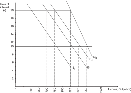
Figure 17.11 The IS Curves Plotted
Y = 1260 – 40r
LM equation will remain unchanged at
Y = 490 + 15r
Simultaneous equilibrium for the IS curve and LM curve
IS = LM
1260 – 40r = 490 + 15r
15r + 40r = 1260 – 490
55r = 770
r = 14%
Y = 1260 – 40 × 14
Y = 700
Simultaneous equilibrium for the IS curve and LM curves exists when Y = 700 and r = 14%.
Solution 3
- Equation of the goods market equilibrium or the IS curve (i) Y = C + I + G
Y = 50 + 0.6Yd + 200 – 5r + 130
Y = 50 + 0.6(Y – 0) + 200 – 5r + 130
Y = 50 + 0.6Y + 200 – 5r + 130
Y – 0.6Y = 380 – 5r
0.4Y = 380 – 5r
Y = 950 – 12.5r
- Equation of the of the IS curve
- Government expenditure increases by Rs. 50 crores
Y = C + I + G
Y = 50 + 0.6(Y – 0) + 200 – 5r + 180
Y = 50 + 0.6 (Y – 0) + 200 – 5r + 180
Y = 50 + 0.6Y + 200 – 5r + 180
Y – 0.6Y = 430 – 5r
0.4Y = 430 – 5r
Y = 1075 – 12.5r
- Taxes increases by Rs. 50 crores
Y = C + I + G
Y = 50 + 0.6(Y – 50) + 200 – 5r + 130
Y = 50 + 0.6(Y – 50) + 200 – 5r + 130
Y = 50 + 0.6Y – 30 + 200 – 5r + 130
Y – 0.6Y = 350 – 5r
0.4Y = 350 – 5r
Y = 875 – 12.5r
- Government expenditure increases by Rs. 50 crores and taxes increases by Rs. 50 crores. This is the case of the balanced budget.
Y = C + I + G
Y = 50 + 0.6(Y – 50) + 200 – 5r + 180
Y = 50 + 0.6(Y – 50) + 200 – 5r + 180
Y = 50 + 0.6Y – 30 + 200 – 5r + 180
Y – 0.6Y = 400 – 5r
0.4Y = 400 – 5r
Y = 1000 – 12.5r
- In Figure 17.11,
- The initial IS curve, Y = 950 = 12.5r is given by the curve IS1
(a) The IS curve when government expenditure increases by Rs. 50 crores, Y = 1075 – 12.5r is given by the curve IS2. This indicates a horizontal shift of Rs. 125 crores.
(b) The IS curve when taxes increase by Rs. 50 crores, Y = 875 – 12.5r is given by the curve IS3. This indicates a horizontal shift towards the left of Rs. 75 crores from the IS1 curve.
(c) The IS curve when government expenditure increases by Rs. 50 crores and taxes increase by Rs. 50 crores, Y = 1000 – 12.5r, given by the curve IS4. This indicates a horizontal shift towards the right of Rs. 50 crores. This is because ΔG = ΔT = 50 crores.
- Government expenditure increases by Rs. 50 crores
Solution 4
- Equation of the goods market or the IS curve
Y = C + I + G
Y = 1000 + 0.80(Y – 0.25Y) + 1500 – 60r + 1000
Y = 1000 + 0.80(0.75Y) + 1500 – 60r + Rs. 1000
Y = Rs. 3500 + 0.6Y – 60r
Y = Rs. 8750 – 150r
- Equation of the money market or the LM curve:
M = L
Y = 7500 + 100r
- Simultaneous equilibrium for the IS and LM curves
IS = LM


Subtracting Eq. (2) from (1), we get
0 = 1250 – 250r
r = 5%
Y = Rs. 8000
Solution 5
Equation of the IS curve
Y = C + I + G
Y = 200 + 0.80Yd + 250 – 7.2r + 90
Y = 200 + 0.80(Y – T) + 250 – 7.2r + 90
Y = 200 + 0.80(Y – 0.20Y) + 250 – 7.2r + 90
Y = 200 + 0.80Y – 0.16Y + 340 – 7.2r
Y – 0.80Y + 0.16Y = 540 – 7.2r
0.36Y = 540 – 7.2r
Y = 1500 – 20r
Equation of the LM curve
ms = 180
md = 0.2Y – 2r
In equilibrium, md = ms.
Thus,
0.2Y – 2r = 180
0.2Y = 180 + 2r
Y = 900 + 10r
Simultaneous equilibrium for the IS curve and LM curves
IS = LM
1500 – 20r = 900 + 10r
20r + 10r = 1500 – 900
30r = 600
r = 20%
Y = 1100
Simultaneous equilibrium for the IS curve and LM curves exists when Y = 1100 and r = 20%.
UNSOLVED NUMERICAL PROBLEMS
-
(a) Equation of the goods market equilibrium or the IS curve
Y = 11000(b) Equation of the money-market equilibrium or the LM curve
Y = 10500 + 500r(c) The equilibrium income and the interest rate:
Y = 11000
r = 1%Simultaneous equilibrium for the IS curve and LM curves exists when Y = 11000 and r = 1%.
-
(a) Equation of the IS curve
Y = 2400 – 25r(b) Equation of the LM curve
Y = 2000(c) Simultaneous equilibrium for the IS curve and LM curves
r = 16%
Y = 2000(d) Simultaneous equilibrium for the IS curve and LM curves exists when Y = 2000 and r = 16%.
I = 200 -
(a) Equation of the IS curve when government expenditure increases by Rs. 20 crores
Y = 2500 – 25r(b) Equation of the LM curve
Y = 2000
Hence, the equation of the LM curve remains unchanged as there is no change in the demand and supply of money.(c) The equilibrium income level and the rate of interest
r = 20%
Y = 2000(d) Simultaneous equilibrium for the IS curve and LM curves exists when Y = 2000 and r = 20%.
I = 180 -
(a) Equation of the IS curve
Y = 900 – 25r(b) Equation of the LM curve
Y = 550 + 25rSimultaneous equilibrium for the IS curve and LM curves.
r = 7 %
Y = 725Simultaneous equilibrium for the IS curve and LM curves exists when Y = 725 and r = 7%.
(c) Equilibrium of the economy if G increases from 100 to 200
Equation of the IS curve
Y = 1150 – 25r
Equation of the LM curve
Y = 550 + 25r
Simultaneous equilibrium for the IS curve and LM curves.
r = 12%
Y = 850Simultaneous equilibrium for the IS curve and LM curves exists when Y = 850 and r = 12%.
- Equation of the IS curve
Y = 1000 – 15r
Equation of the LM curve
Y = 400 + 25r
Simultaneous equilibrium for the IS curve and LM curves.
r = 15%
Y = 775
Simultaneous equilibrium for the IS curve and LM curves exists when Y = 775 and r = 15%.