Chapter 2 The Derivative

2.1 The Limit

• This section includes a summary of the limit, its applications, conditions for estimating an infinite series, and convergence.

• The limit is used in the estimation of infinite sums and in the definitions of the derivative and the integral. In general, the limit is used to describe closeness of a function to a value when the exact value cannot be identified. The limit is also used to determine if functions are continuous or discontinuous. Whether the graph of a given function is a smooth and continuous curve or line, or whether there are breaks or holes present can be determined using the limit.

• If the lim_x→a f(x) = L, then it is said that the function f(x) gets close to and may equal some number L as x approaches and gets close to some number a.

• Consider a simple example where the limit as x approaches 1 is taken of function f(x) = x² + 2:

lim_x→1 f(x) = lim_x→1(x² + 2)

By substituting numbers for x that get closer to the number 1, it can be shown that as x gets closer to 1, or lim_x→1, then x² gets closer to 1 and f(x) gets closer to 3.

• In more complicated examples, simply substituting the desired number into the function is not possible. For example, consider the limit:

lim_x→2[(x² − 4) / (x − 2)]

If x = 2 is substituted into this equation, the result is 0/0, which is undefined. In this equation, factoring can be used to determine if the limit exists. (See Section 5.7 in Master Math: Algebra for a review of factoring polynomials.)

The factoring of [(x² − 4) / (x − 2)] results in: x + 2.

Taking the limit results in: lim_x→2(x + 2) = 4.

Therefore, as x gets close to 2, then x + 2 gets close to 4.

• There are many cases where the limit of a function does not exist. For example, consider the limit as y gets close to zero for the function f(y) = 1/y: lim_y→0(1/y).

Because 1/0 is undefined, it is possible to substitute values for y approaching zero:

If y = 0.1, f(y) = 1/0.1 = 10

If y = 0.01, f(y) = 1/0.01 = 100

If y = 0.001, f(y) = 1/0.001 = 1,000

If y = − 0.01, f(y) = 1/−0.01 = −100

If y = −0.001, f(y) = 1/−0.001 = −1,000

As y gets close to 0, 1/y does not get closer to any number. The magnitude of 1/y actually increases. Therefore, lim_y→0(1/y) approaches ∞, and the limit does not exist.

• If the limits of the functions f(x) and g(x) exist, then the rules governing limits of functions that are added, subtracted, multiplied, divided, and raised to a power are:

lim_x→a(f(x) + g(x)) = lim_x→a f(x) + lim_x→a g(x)

lim_x→a(f(x) − g(x)) = lim_x→a f(x) − lim_x→a g(x)

lim_x→a(f(x) × g(x)) = lim_x→a f(x) × lim_x→a g(x)

lim_x→a(f(x) ÷ g(x)) = lim_x→a f(x) ÷ lim_x→a g(x), if lim_x→a g(x) ≠ 0

lim_x→a(f(x))^y = (lim_x→a f(x))^y

• The limit can be used to estimate the sum of an infinite series. If the progression or sequence is infinite and therefore there is an infinite number of terms, then the sum cannot be calculated. However, under certain conditions the sum of an infinite series can be estimated.

• Conditions that determine if the sum of an infinite series can be estimated include the following.

(a.) If an infinite series has a limit, it is said to converge and the sum can be estimated. In other words, as the terms in an infinite series are added, beginning with the first term, if with each additional term added the sum approaches some number, then the series has a limit and converges and the sum can be estimated.

(b.) A condition for convergence for the infinite series:

is that a_n must approach zero as n approaches infinity. Although this condition must occur for a series to converge, there are cases where this condition is true but the series still diverges.

(c.) If an infinite series has no limit, it is said to diverge and the sum cannot be estimated. In other words, if instead as each additional term is added the sum approaches infinity, then the series has no limit and diverges and the sum cannot be estimated.

• To estimate an infinite series, it must be determined whether the series has a limit and converges and what happens to the sum as the number of terms approach infinity. For an infinite series describing the sum of a_n from n = 1 to n = ∞:

If this series has a limit and converges to L it becomes:

For convergence to zero, the values of a_n must become small at some small number and remain below that number. The small number may be on the order of 10^-10, etc. The generally accepted notation for representing this small number that a converging sequence will approach and remain below is ε (Epsilon). The general rule is, for any value of ε, there is a number N where | a_n | < ε if n > N.

For convergence to numbers other than zero, the general rule is, for any ε, there is a number N where | a_n − L | < ε if n > N. In this case, lim_n→∞ a_n = L. Convergence occurs when values for a_n approach L and remain in a range of L + ε and L − ε.

• When two sequences, a_n and b_n, each converge such that lim_n→∞ a_n = L and lim_n→∞ b_n = L*, then the following are true:

lim_n→∞(a_n + b_n) = L + L*

lim_n→∞(a_n − b_n) = L − L*

lim_n→∞(a_n b_n) = L L*

lim_n→∞(a_n/b_n) = L/L* provided L*≠ 0

2.2 Continuity

• This section provides a brief summary of continuity including the definition of a continuous function, a continuable function, examples of continuous functions, discontinuous functions, conditions of discontinuity, and visualizing continuity.

• A function is considered continuous at x = a, if lim_x→a exists, such that the lim_x→a f(x) = f(a) and f(a) is defined. If f(x) is continuous at x = a, then f(x) → f(a) as x → a. For a function to be defined as a continuous function, it must be continuous at every point where it is defined.

• A function is called continuable if the definition of continuous can be applied to all x values such that the function is continuous at all x values. For example, f(x) = 1/x is not continuable but is continuous by definition because it is“not defined" at 1/x where x = 0. A function is continuous at x if as ∆x → 0, then [f(x + ∆x) − f(x)] → 0, where ∆x represents some small change or increment in x.

• A polynomial function is an example of a continuous function that is continuous everywhere and its graph is a continuous curve. (With the exception of ratios of polynomial functions with zero denominators.)

Other continuous functions include exponential, sine, cosine, and rational functions on intervals where their denominators are not zero.

• A function that is not continuous may be discontinuous at a single point. For example, the function f(x) = 1/x is continuous except at x = 0 where 1/0 is undefined. Therefore, lim_x→a f(x) = lim_x→a1/x = 1/a. In general, the graph of a continuous function has no holes or breaks.

• The following graphs are of (a.) a function that is discontinuous at a point, (b.) a function that is discontinuous at more than one point and has a jump, (c.) function f(x) = 1/x², and (d.) function f(x) = 1/x:

• The following are conditions where discontinuity exists:

(a.) If lim_x→a f(x) exists and is equal to L, but f(x) does not exist when x = a so that f(a) ≠ L, then the graph of f(x) is discontinuous at the point x = a. In this case there is only discontinuity at a single point.

(b.) If lim_x→a f(x) does not exist because as x approaches a from either x > a or x < a, the value of f(x) approached from x > a is different from the value f(x) approached from x < a, then the graph of f(x) is discontinuous and has a jump at point a = x.

(c.) If lim_x→a f(x) does not exist because as x approaches a, the absolute value |f(x)| gets larger and larger then the graph is“infinitely discontinuous”at x = a.

• A means to visualize whether a function is continuous involves use of symbols such as Epsilon ε and Delta δ to define regions in question on the X and Y axes of the graph of a function. Consider the limit of the function f(x) where lim_x→a f(x) = L, and has the following properties:

(a.) The limit exists.

(b.) ε represents an error tolerance allowed for L.

(c.) δ represents the distance that x is from x = a.

In this graph a value for ε can be chosen and δ(ε) results. Conversely, a value for δ can be chosen and ε(δ) results.

As lim_x→a f(x) = f(a) = L, providing the limit exists, where:

L + ε = f(a) + ε, or L = f(a), also L − ε = f(a) − ε,

then the following is true:

f(a) + ε > f(x) > f(a) − ε, or equivalently, | f(x) − L | < ε.

For every chosen number ε where ε > 0, there is a positive number for δ(ε) that results.

For a chosen f(x), x must be within (a − δ) and (a + δ) such that a − δ < x < a + δ, or equivalently, 0 < | x − a | < δ.

Therefore, as x gets close enough to a, then | f(x) − L | < ε, and the closeness of x is defined to have a tolerance of δ such that when 0 < | x − a | < δ then | f(x) − L | < ε.

2.3 Differentiability

• This section summarizes the concept of differentiability. (See the next section for the definition of the derivative.)

• A function is differentiable at any point where it has a derivative. A function that has a derivative at every point is differentiable everywhere. At any point where f(x) has a derivative, the function is continuous. There can be a point where f(x) is continuous but no derivative exists, such as where the graph turns a corner without a hole or jump.

• A graph of a function has a derivative and is therefore differentiable at a point if a tangent line can be drawn at that point.

• If for a given point on the graph of a function the derivative does not exist, then that point may be (a.) at the end of the curve of the function; (b.) at a corner on the curve; (c.) at a location where the tangent line is a vertical line and therefore has no slope; or (d.) at a location on the graph that is discontinuous such as if one point is missing or there is a jump in the curve of the function.

2.4 The Definition of the Derivative and Rate of Change

• This section includes the definition of the derivative, notation, developing the definition of the derivative, calculating velocity using the derivative, the average rate of change, and the instantaneous rate of change.

• The derivative is used to describe the rate of change of something such as velocity, as well as the concept of the tangent to a curve. Applications of the derivative include tangents, slopes, rates of change, curvilinear and straightline motion, maxima, minima, and tests for extrema.

• Notation for the derivative of a function f(x) includes:

If y = f(x) then the derivative f′(x) can be written (dy/dx).

Notation for taking second derivatives includes:

Notation for the nth derivative includes:

• The time rate of change of an object in motion such as a car, plane, pitcher’s fast ball, etc., is the rate of change of distance with respect to time and is called velocity. The velocity is the derivative or equivalently the rate of change of distance with respect to time. Velocity can be positive or negative with respect to a reference point, but speed is the magnitude of velocity and is always positive or zero.

• To consider rate of change, remember that distance equals rate times time, d = rt, therefore, rate = (distance / time).

The time rate of change of distance is velocity and average velocity = (change in distance / change in time).

Also, the time rate of change of velocity is acceleration and acceleration = (change in velocity / change in time).

• To develop the definition of the derivative, consider the velocity of an airplane flying from the east coast to the west coast.

The distance the airplane is from its starting point or any defined reference point is a function of time (depends on time) or f(t). (In this example, f is the distance function.)

At time = t, the airplane is f(t) units from the starting or reference point. (The units could be hours.)

At time = t + h, the airplane is f(t+h) units from the starting or reference point and h represents an increment of time.

The change in the position of the airplane during the increment of time h is f(t+h) − f(t).

The rate of change of the distance with respect to time between time = t and time = t+h is the average velocity of the airplane. The average velocity during this time period is:

To find the velocity of the airplane at a particular point when time = t, shrink the time increment h surrounding time t. The velocity at the point where time = t is called the instantaneous velocity, and is determined by taking the limit as the increment of time h shrinks to zero:

velocity at time

As h gets close to zero (but not equal to zero), the time increment h and the distance f(t+ h) − f(t) will get smaller.

Because velocity is the derivative of distance, then the definition of the derivative with respect to time of the distance function f(t) can be written:

, provided the limit exists.

• The velocity at time t or v(t) can be determined using the definition of the derivative and the following procedure:

(a.) Determine f(t+h) and f(t).

(b.) Subtract f(t) from f(t+h).

(c.) Divide [f(t+h) − f(t)] by h.

(d.) Take the limit as h approaches zero.

• Example: Find the velocity at t = 2 hours, if the distance in miles is represented by f(t) = 3t².

f(t+h) = 3(2 + h)² = 3(4 + 4h + h²) = 12 + 12h + 3h²

f(t) = 3(2)² = 12

f(t+h) − f(t) = (12 + 12h + 3h²) − 12 = 12h + 3h²

(f(t+h) − f(t)) ÷ h = (12h + 3h²) ÷ h = (12h)/h + (3h²)/h = 12 + 3h

lim_h→0(12 + 3h) = 12 = the velocity at 2 hours, v(2hrs)

Therefore, the velocity at t = 2 hours is 12 miles/hour.

• The definition of the derivative with respect to x, rather than with respect to time, can be written:

• It is possible to use the definition of the derivative to determine the average rate of change or the instantaneous rate of change of a function. In general, the rate of change represents how fast or slow a function changes from one end of the interval to the other end, relative to the size of the interval (given by h).

• The average rate of change of f over an interval from some value of x to some value of x + h is given by:

The average rate of change is equivalent to the slope of a line drawn between two points on the graph of a function f(x) represented by x values between the value of x = a to the value of x = (a + h).

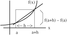
• The instantaneous rate of change of f(x) at some point x is given by the following expression, which represents the average rate of change over smaller and smaller intervals. This expression defines the derivative of f at some point x.

The instantaneous rate of change is equal to the slope of the graph of the function at some point on the curve, or equivalently the instantaneous rate of change is equal to the slope of a line drawn tangent to the curve at that point.

2.5 Δ (delta) Notation and the Definition of the Derivative

• This section introduces delta Δ notation for the definition of the derivative.

• An alternative notation for writing the definition of the derivative is to use Δx in place of h and Δy (or Δf) in place of f(x + Δx) − f(x). Using this Δ (delta) notation the derivative with respect to x can be written:

In the context of an XY coordinate system, Δy/Δx represents the average rate of change of y per unit change in x over the interval of a curve of a function between x and x +Δx. Similarly, dy/dx represents the instantaneous rate of change in y per unit change in x at some point (x,f(x)).

This is also sometimes written:

• Distance and time are sometimes represented using the definition of the derivative as:

where Δt represents a small increment of time, such that the distance at some time (t + Δt) is represented by f(t + Δt). The distance at time t is represented by f(t) and the change in distance is Δf = f(t + Δt) − f(t). The average velocity is the change in distance Δf divided by the change in time Δt, or Δf/Δt. The instantaneous velocity at a given time is found by shrinking Δt by taking the limit as Δt→0, which is f′(t) or df/dt. The average slope of the graph of f is Δf/Δt, and the slope at some point t on the graph of f is df/dt.

• For example, if a car is driving at a constant velocity of 65 mi/hr, the distance the car travels is given by f = d = vt. The distance traveled at any time t is f = vt, and at a later time (t + Δt) is v(t + Δt). The velocity can be represented by Δf/Δt. If Δf = vΔt is substituted, velocity becomes Δf/Δt = vΔt/Δt = v, where lim_Δt→0Δf/Δt = df/dt = v. In 1 hour, the car has traveled 65 miles = 65(1), at 2 hours, 130 miles, etc. Because the car is traveling at a constant velocity, Δf/Δt = df/dt = 65 mi/hr, and the limit is not required.

• Various notations are used to represent functions. It is important to understand what is being described and stay consistent with the notation within a given problem.

2.6 Slope of a Tangent Line and the Definition of the Derivative

• This section includes the slope of a tangent line and the definition of the derivative, and the equations for a tangent line, a secant line, and a normal line.

• In the graph of a function, the slope of a line drawn tangent to the curve through some point (a,f(a)) on the curve is the derivative of the function at point (a,f(a)). In other words, the slope of the tangent at point (a,f(a)) equals the derivative f′(a) at that point. (If a tangent line is vertical, its slope is undefined.) The slope of a tangent at a point measures the change in the curve at that point.

• The definition of the derivative can be used to prove that the slope of a line drawn tangent to a graph of a function at some point, is the derivative of the function at that point. Consider the two points on the curve (a,f(a)) and (a+h,f(a+ h)). Tangent 1 is drawn through point (a,f(a)), tangent 2 is drawn through point (a+h,f(a+ h)), and a “center line” is drawn through the two tangent points.

The slope of the center line through point (a,f(a)) and point (a+ h,f(a+ h)) represents the change in y over the change in x between the two points and is equal to:

If the value of the increment h between the two points is reduced, the value of h will approach zero, and the tangent 2 line through point (a+ h,f(a+ h)) will approach being equal to the tangent 1 line through point (a,f(a)). Therefore, the slope of the tangent at point (a,f(a)) equals the derivative f′(a):

= the slope of tangent 1

provided the limit exists.

Therefore, the slope of the tangent at (a,f(a)) is the derivative of f at point a.

• Note that the derivative at a point on a curve can be represented as either the slope of the tangent line to the curve at that point, or the slope of the curve at that point.

• The equation for the tangent line at y = f(x) and x = a is:

y − f(a) = f′(a)(x − a)

This can be derived as follows:

f (a)(h) ≈ f(a + h) − f(a)

f(a + h) ≈ f′(a)(h) + f(a)

where if x − a = h and x = a + h,

f(a + h) ≈ f′(a)(x − a) + f(a)

f(x) ≈ f′(a)(x − a) + f(a)

using y = f(x),

y − f(a) = f′(a)(x − a)

This is used to linearize and estimate a region of f(x) close to x = a near the point (a,f(a)) on a curved function.

• The secant line is represented by a line drawn between two points on a curve. The equation for the secant line is:

The slope of the secant line, f′(x₁), is given by:

A secant line becomes a tangent line by letting x = x₂ approach x = x₁:

• Another important equation is the equation for a line normal or perpendicular to the tangent line on a curve at a given point. The slope of the tangent line and slope of a perpendicular line multiply to equal − 1. If m is the tangent line and − 1/m is the normal line, then the equation for the normal line can be written:

y − y₁ = (-1/m)(x − x₁) or y − f(a) = [-1/f′(a)](x − a)

2.7 Velocity, Distance, Slope, Area, and the Definition of the Derivative

• This section includes a summary of the relationship between velocity and distance; increasing velocity; constant velocity; and velocity, distance, and the area under a curve.

• The relationship between distance traveled f and velocity v is such that if f is known, v can be obtained, and if v is known, f can be obtained. Finding velocity from distance traveled involves differentiation and finding distance traveled from velocity involves integration. (Integration is discussed at length in Chapter 3.)

• Consider the graphs below of f(t) = 3t². Values of v(t) can be calculated for various t values using the definition of the derivative by (a.) determining f(t+h) and f(t); (b.) subtracting f(t) from f(t+h); (c.) dividing [f(t+h) − f(t)] by h; and (d.) taking the limit as h approaches zero, lim_h→0.

Using these four steps for f(t) = 3t², v(t) for t = 2 was calculated in Section 2.4 to be v(2) = 12. Using these same four steps for other values of t, t = 0, 1, 3, results in v values of v(0) = 0, v(1) = 6, and v(3) = 18. In summary:

f(0) = 0, v(0) = 0

f(1) = 3, v(1) = 6

f(2) = 12, v(2) = 12

f(3) = 27, v(3) = 18

In this example, the velocity is increasing with distance and time. The slope of the curve drawn for f(t) is equal to v(t) at each point. Therefore, if a tangent line is drawn at each point for t, its slope is the velocity at that point or v(t). Note that the slope of v(t) is the acceleration.

• If velocity v remains constant, f will increase at that constant rate and f = vt. For example, if v(t) = 6 mi/h, then f = 6t. Therefore, for:

t = 1, f = 6

t = 2, f = 12

t = 3, f = 18

v(t) is constant at 6 since the slope of f(t) is the same and equal to 6 at every point t.

• The graph for v can be determined by calculating the slope of the f graph. When the slope of f is a straight line, the velocity is constant, and the graph of v(t) is a straight horizontal line at the constant slope value for f(t). When f is a curve, the slope must be calculated at each point by determining the slope of a tangent line drawn at each point. The slope can be positive or negative depending on whether the velocity or rate-of-change is increasing or decreasing (accelerating or decelerating).

• To determine f from v graphically, it turns out that the area under the curve (or line) of v gives f. Therefore, the area under a graph of velocity represents the value for distance. This is discussed in Chapter 3. For a constant v the area is the rectangular region under v with height = v, width = t, and area = vt. This is consistent with f = vt. The area under v is a sum of areas at each t value that corresponds to distances at each time increment. For sloped or curved v graphs, the area can also be divided into incremental areas at each t value, where the velocity within each small increment is nearly constant.

• If a set of f values is listed, the differences between f’s are v values. For example, if f = 1, 4, 8, 10, 12, then taking the difference between each f value results in a list of differences or v values, v = 3, 4, 2, 2. The sum of the differences in f values is 3 + 4 + 2 + 2 = 11, which is equivalent to the difference between the first and last f value 12 − 1 = 11. Therefore, the v values are the differences in f values at defined increments, and the area under v is the sum of the increments. The difference between the first and last value of f is:

area = f(t_last) − f(t_first), or,

(f₁ − f₀) + (f₂ − f₁) + (f₃ − f₂) + (f₄ − f₃) + ... = f_n − f₀

= v₁ + v₂ + v₃ + ... + v_n

• For example, consider a sine wave type of pattern where the curve oscillates from positive to negative to positive, and so on. Values of f follow the pattern:

f = 0, 1, 1, 0, -1, -1, 0

where the differences which correspond to v values are:

v = 1, 0, -1, -1, 0, 1

The area is:

f(t_last) − f(t_first) = 0 = sum of the differences (v values)

Suppose more values are added:

f = 0, 1, 1, 0, -1, -1, 0, 1, 1, the differences are:

v = 1, 0, -1, -1, 0, 1, 1, 0

f(t_last) − f(t_first) = 1 = sum of the differences (v values)

The area of v is the sum of the incremental positive and negative areas over a chosen interval of corresponding f and v values.

• For example, consider f = 1, 2, 3, 4, 5, 6. The differences are v = 1, 1, 1, 1, 1. The sum of the differences of the increments is: f(t_last) − f(t_first) = 5.

Slope of f = 1 = v, and area under v is f(t_last) − f(t_first) = 5.

2.8 Evaluating Derivatives of Constants and Linear Functions

• This section includes the derivative of a constant or a constant function and the derivative of a linear function. (The derivative of a constant multiplied by a variable is discussed in Section 2.10.)

• The derivative is the rate of change of something that is changing, therefore the derivative of a constant is zero. The derivative of constant function f(x) = c is zero everywhere, because its graph is a horizontal line with a slope of zero everywhere. In the graph below, f(x) = c is a constant function with a slope of zero, therefore f′(x) = 0.

• The rate of change of a linear function is constant because for each change in x along the graph of a linear function, the corresponding changes in y are the same. The graph of a linear function is a straight line and the slope of a straight line is constant, therefore the rate of change or derivative of a linear function is constant.

Remember the equation for a line is f(x) = mx + b, where the constant slope is m = derivative = f′(x). Calculating the derivative of f(x) = mx + b using the derivative formula (derived in the following section) is:

df(x)/dx = d(mx)/dx + db/dx = m + 0 = m

where m represents the constant slope of the straight line that represents the function.

2.9 Evaluating Derivatives Using the Derivative Formula

• This section introduces the derivative formula including its derivation.

• Evaluating derivatives using the definition of the derivative is laborintensive. Instead, there is a shortcut formula used to evaluate derivatives. This derivative formula is:

where x represents any variable and n is any number.

• If a constant a is multiplied by the variable xⁿ, the derivative formula becomes:

Note: The derivative formula is important and used frequently in calculus.

• The derivative formula can be derived from the definition of the derivative as follows:

Consider a function f(x) = axⁿ where a is some constant, x is a variable, and n is a number.

Substitute this function into the definition of the derivative:

Factor out the constant a:

The (x + h)ⁿ term can be expanded using the binomial expansion:

Because there are no h², h³, etc., terms in the definition of the derivative, and the limit as h→0 will quickly remove these, write the binomial expansion excluding the h² and greater terms. This expansion becomes:

(x + h)ⁿ = xⁿ + nx^n-1h

Substitute the expansion for (x + h)ⁿ into the definition of the derivative:

Cancel the xⁿ terms:

Factor and cancel an h from each term:

lim_h→0 a(nx^n-1)

Therefore, as h→0:

This is the derivative formula.

2.10 The Derivatives of a Variable, a Constant with a Variable, a Constant with a Function, and a Variable Raised to a Power

• In this section, the derivative formula is applied to

f(x) = x, f(x) = cx, and f(x) = cxⁿ.

• The derivative of an independent variable x with respect to itself is one.

• The derivative of a constant c times an independent variable x with respect to x is equivalent to the constant times the derivative of the independent variable.

• The derivative of a constant times a function f(x) is equivalent to the constant times the derivative of the function.

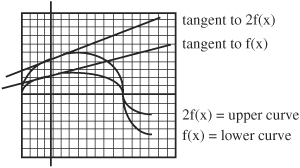
• By multiplying a function by a constant, the graph of that function will be affected by the constant. The graph will have the same general shape as it does without the multiple. However, it may have a larger or smaller amplitude, it may be elongated or narrower, it may be moved to the right or left or up or down, or if multiplied by a negative constant it may be flipped over the X-axis.

The slopes (or derivatives) of the curve of the graph of a function multiplied by a constant will be different at each point along the curve from the slopes of the curve of the original function. The change in the slopes will be proportional to the value of the constant.

For example, if a function is multiplied by the constant 2, the amplitude of the graph will be two times the amplitude of the original graph. Similarly, if a function is multiplied by the constant 1/2, the amplitude of the graph will be one-half the amplitude of the original graph.

• The derivative of a function with the variable raised to a power in the form cxⁿ evaluated using the derivative formula is:

where c represents any constant number that may be multiplied with the function and n is an integer.

For example, (d/dx)3x² = (3)(2)x^2-1 = 6x

If n is negative the formula becomes:

2.11 Examples of Differentiating Using the Derivative Formula

• This section includes using the derivative formula to evaluate simple functions and calculating the derivative of 1/x using the definition of the derivative as a comparison.

• The following are examples of using the derivative formula to evaluate derivatives:

• Using the derivative formula to evaluate (d/dx)(1/x) resulted in − 1/x². Evaluate this derivative using the definition of the derivative and compare the results:

Using , gives:

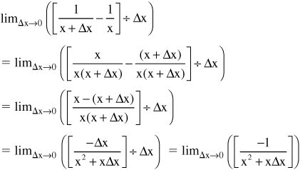
as Δx→0, this approaches − 1/x², which is the same answer obtained using the derivative formula.

2.12 Derivatives of Powers of Functions

• This section includes evaluating powers of functions using the derivative formula, comparing results with the definition of the derivative and graphs.

• To evaluate the derivatives of powers of functions, the derivative formula can be applied to the whole function, which is then multiplied with the derivative of what is inside. This is known as the chain rule and is discussed in Section 2.19.

• Results obtained using this method can be compared with results obtained using the definition of the derivative. For example, if (d/dx)(f(x))²:

Remember the factored form of (x² − y²) is (x + y)(x − y). Using this for Δf:

therefore,

• Following are graphs of functions raised to a power and their derivatives.

Example: If f(x) = x³, using the derivative formula results in 3x². The graph of x³ and its derivative is represented as:

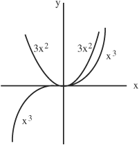
Example: If f(x) = x², using the derivative formula results in 2x. The graph of x² and its derivative is:

Because the derivative of x² is 2x, which is a linear function, the graph of the derivative is a straight line with a constant slope of 2.

2.13 Derivatives of a^x, e^x, and ln x

• This section includes calculating derivatives along a curve of a^x, demonstrating that the derivative of e^x is e^x, the relationship between the derivative of a^x and the natural logarithm, and the derivative of the natural logarithm and of functions that involve the natural logarithm.

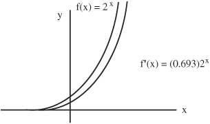
• Graphs of exponential functions in the form f(x) = e^x and f(x) = a^x, depict that for negative values of x, f(x) increases slowly and for positive values of x, f(x) increases faster.

For real values of x, the graph of the derivative of f(x) = a^x exists above the X-axis.

• Consider f(x) = a^x when a = 2. The curve of f(x) = 2^x can be plotted by selecting x values and solving for f(x):

x = −3, f(x) = 2^-3 = 1/2³ = 1/8

x = −2, f(x) = 2^-2 = 1/2² = 1/4

x = −1, f(x) = 2^-1 = 1/2¹ = 1/2

x = −0, f(x) = 2⁰ = 1

x = 1, f(x) = 2¹ = 2

x = 2, f(x) = 2² = 4

x = 3, f(x) = 2³ = 8

x = 4, f(x) = 2⁴ = 16

It is possible to calculate the derivative for f(x) = 2^x at points along the curve using the definition of the derivative. This can be developed by first applying the definition of the derivative to the general case of a^x and developing a general formula. Begin with:

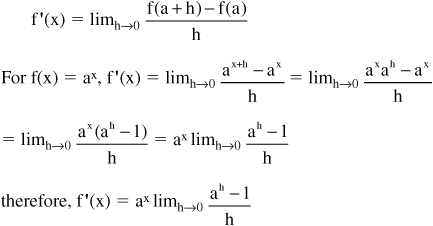
This formula shows that the derivative of a^x is equal to a^x multiplied by the limit of a constant. This expression for f′(x) can then be used to calculate values of the slope and, thus, the derivative of a^x at various points along the curve. Using this formula to calculate the derivative for f(x) = 2^x, where a = 2, first select x values along the curve such as x = −1, x = 0, and x = 1, and apply the formula:

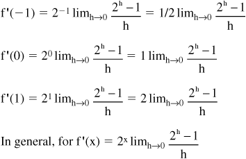
Taking the limit as h→0, by choosing small h values to see what the value of (2^h − 1) / h approaches:

h = −0.001, the limit = 0.692907

h = +0.001, the limit = 0.693387

h = −0.0002, the limit = 0.693099

h = +0.0002, the limit = 0.693195

h = −0.0001, the limit = 0.693123

h = +0.0001, the limit = 0.693171

Therefore, as h→0, (2^h − 1) / h approaches 0.6931.

The derivative of f(x) = 2^x can be calculated using:

(d/dx)2^x = 2^x(0.6931)

It is then possible to use this resulting formula to calculate the derivative at various points along the curve of 2^x for different x values such as x = −1, 0, 1:

f′(-1) = 2^-1lim_h→0(2^h − 1) / h = 2^-1(0.6931) = 1/2(0.6931) = 0.346

f′(0) = 2⁰lim_h→0(2^h − 1) / h = 2⁰(0.6931) = 1(0.6931) = 0.693

f′(1) = 2¹lim_h→0(2^h − 1) / h = 2¹(0.6931) = 2(0.6931) = 1.386

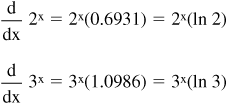
• Consider f(x) = a^x where a = e. The general expression f′(x) = a^xlim_h→0(a^h − 1) / h developed in the preceding paragraphs can be used to show that the derivative of e^x is e^x. To show that the derivative of e^x is equal to the original function e^x, first notice that the quantity lim_h→0(a^h − 1) / h does not depend on the value of x and is therefore a constant for each unique value of a. It was calculated in the preceding paragraphs that this quantity of the limit is 0.6931 when a = 2 and therefore f′(x) = 2^x(0.6931).

Similarly, it can be calculated using the same process that the quantity of the limit is 1.0986 when a = 3, and therefore f′(x) = 3^x(1.0986). Notice that when a = 2, the quantity of the limit is less than 1 and the derivative of a^x is slightly less than the original function a^x. Also, when a = 3, the quantity of the limit is greater than 1 and the derivative of a^x is slightly greater than the original function a^x.

Expanding on this and using these observations in combination with the fact that e = 2.7818, the quantity of the limit must be equal to 1. This is consistent with the fact that the derivative of e^x must be equal to the original function e^x.

It is possible to find the value of a when a = e, which is the number that e represents, using this quantity of the limit where it is equal to 1:

lim_h→0(a^h − 1) / h = 1

First isolate a by considering the quantity of the limit at small h values:

(a^h- 1) / h ≈ 1

a^h − 1 ≈ h

a^h ≈ h + 1

a ≈ (h + 1)^1/h

Select small values for h as h→0:

h = 0.0001, a ≈ 2.7181

h = −0.0001, a ≈ 2.7184

h = 0.00001, a ≈ 2.7183

h = −0.00001, a ≈ 2.7183

These values of a = e converge to a = e = 2.71828...

By substituting e = 2.718 and choosing small h values, it can be shown that: lim_h→0(e^h − 1) / h = 1

Therefore, (d/dx)e^x = e^x

Note that the slope at x = 0 is one.

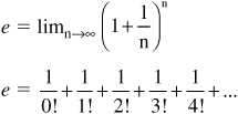
• Note that e can be expressed in the following two forms:

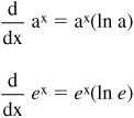
• The exponential function is related to the natural logarithm such that ln (e^x) = x and e^lnx = x. In the examples of the derivatives of a^x where a = 2 and a = 3, the quantities of the limits are 0.6931 and 1.0986, respectively. These values are natural logarithms, such that 0.6931 − ln 2 and 1.0986 − ln 3. Therefore, using the formula developed in the preceding paragraphs:

Similarly, the following derivatives can be written:

• The derivative of the natural logarithm of x, or ln x, is 1/x. This can be verified using exponential form and the fact that x = e^{ln x} when x > 0 as follows:

Begin by differentiating both sides of x = e^{ln x}:

Using the chain rule (described in Section 2.19.) where f(g(x))′ = f′(g(x))(g′(x)), differentiate the right side e^{ln x}, or e^f(x):

Substitute f(x) = ln x:

Set equal to the left side:

Therefore, 1/x = the slope of the graph of ln x.

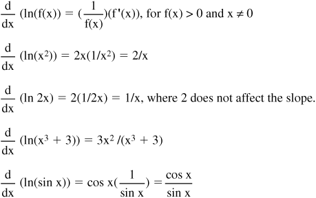
• Following are examples of derivatives that involve the natural logarithm:

2.14 Applications of Exponential Equations

• This section includes the general equation for growth and decay, an example of a bacteria population, and an equation for compound interest.

• There are many questions in science, finance, etc., that can be answered using growth and decay models. For example, the rate of change of growth of a population is often proportional to the size of the population at a given point in time. The general equation for exponential growth and decay is given by the derivative:

dy(t)/dt = ky(t), where

y(t) represents what is growing or decaying at time t (e.g., the size of

a population or the amount of a radioactive substance);

t represents time;

c represents the initial amount (e.g., mass); and

k is a constant of proportionality representing rate of growth or decay,

such that when k > 0 the population is growing at an exponential rate,

and when k < 0 the population is decreasing at an exponential rate.

Differentiating y(t) gives:

Therefore, for any function where dy(t)/dt = ky(t), then y(t) = c e^kt, for some number c.

Note that at t = 0, y(0) = c e^k(0) = c

• Example: Suppose a bacterial population (culture) begins with 100,000 bacteria and in 20 days has 200,000 bacteria. If the population will double in 20 days, how big will it be in 15 days and what is its rate of change in 20 days?

y(t) represents the size of the population in t days

y(t) = ce^kt

First determine c and k:

At t = 0, y(0) = ce^k(0) = c = 100,000

To find k, at t = 20, y(20) = 100,000 e^k(20) = 200,000

Rearranging gives: e^k(20) = 2

Take logarithm of both sides:

ln e^k(20) = ln 2

k(20) = ln 2

k = (ln 2)/20

Substitute c and k into the equation for y(t):

y(t) = (100,000)e^((ln2)/20)t

At t = 15:

y(15) = 100,000 e^{((ln 2)/20)(15)} = (100,000)2^15/20 =

y(15) = 168,179 bacteria in 15 days

The rate of change of the population at 20 days is:

= (ln 2/20)(100,000)e^{(t ln 2)/20}

= (5,000)(ln 2) e^{ln 2} = (5,000)(ln 2)(2) = (10,000) ln 2

= 6,931 bacteria/day

• For examples involving interest on money, the amount of interest earned at a continuously compounded fixed rate will be dependent on the amount of money, and will increase with increasing amounts of money. The growth-decay equation applies to this as well:

y(t) = ce^kt

where y(t) represents the amount of money at time t;

c represents the starting amount;

k represents the continuous or instantaneous growth rate (interest

rate). Note that k is not the same as the annual growth rate.

• Continuously applied compounded interest is sometimes represented by:

P(1+ (i/n))^t

where P represents principal;

t represents number of time periods where amount is checked;

i represents yearly interest rate (decimal form);

n represents number of time periods per year that equal divisions of

the proportional amount of interest is paid; and

i/n represents annual growth rate.

At one year the amount is P(1 + (i/n))ⁿ.

As number of times per year interest is paid increases (such that it is“continuously compounded”):

lim_n→∞ P(1+ (i/n))ⁿ = P lim_n→∞(1 + (i/n))ⁿ

Substitute“in”for n:

P lim_n→∞(1+ (i/in))ⁱⁿ = P lim_n→∞(1 + (1/n))ⁱⁿ

Because e can be expressed as e = lim_n→∞(1 + (1/n))ⁿ, then,

P lim_n→∞(1 + (1/n))ⁱⁿ becomes:

Peⁱ = continuously compounded interest.

2.15 Differentiating Sums, Differences, and Polynomials

• This section includes differentiating sums and differences of functions and differentiating polynomial functions.

• To differentiate functions that are added or subtracted, differentiate each function separately, then add or subtract the resulting functions. If one of the functions contains a polynomial, differentiate the polynomial term by term.

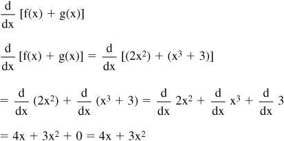
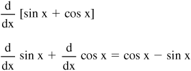
• The sum and difference of the two functions f(x) and g(x) can be differentiated as follows:

• Example: If f(x) = 2x² and g(x) = x³ + 3, find:

• Example: Find:

• Polynomial functions can be differentiated by differentiating each term separately. For example, if x₁, x₂, −x₃, and x₄ each represent a term, then:

Differentiating a polynomial is similar to differentiating a sum or difference:

• For example, differentiate the following polynomial function term by term using the derivative formula:

2.16 Taking Second Derivatives

• This section includes the definition of the second derivative, an example, and notation.

• In general, the second derivative of a function involves taking the derivative of the function that results after the first derivative is taken. The second derivative is the rate of change of the rate of change. For example, velocity v is the rate at which the position of something is changing with respect to time, and acceleration a is the rate at which the velocity is changing with respect to time.

v = dx/dt and a = dv/dt

therefore, a = dv/dt = d²x/dt².

A positive value of a reflects acceleration, and a negative value of a reflects deceleration.

• If y = f(x), the first derivative is f′(x) = dy/dx, then the second

derivative is

• The second derivative provides information about change in slope, the rate of change of something that is changing, such as the growth rate of a population, and is used in minima and maxima problems. (See Section 2.27.)

• To find the second derivative of a function, differentiate the original function first, then differentiate the result. For example, for the polynomial function in Section 2.15,

f(x) = (x³ + 4x² + 7x + 9), the first derivative is 3x² + 8x + 7.

To find the second derivative, differentiate this resulting function:

• Notation for multiple derivatives is:

For the second derivative:

For the nth derivative:

2.17 Derivatives of Products: The Product Rule

• This section includes the definition of the product rule, derivation of the product rule, and the product rule for multiple products.

• The product rule can be used to differentiate the product of two functions. The product rule applied to the product of the two functions f(x) and g(x) is:

Using shorthand notation the product rule is written:

(fg)′ = f′g + fg′

Note: The formula for the product rule is important and used frequently in calculus.

• The product rule can be developed using the definition of the derivative given by:

which can be written for two functions as:

Using the Δ notation and the definition of the derivative, a small change in f, or Δf, is f(x + Δx) − f(x) and a small change in g, or Δg is g(x + Δx) − g(x), such that:

Because, Δf = f(x + Δx) − f(x)

rearrange:

f(x + Δx) = Δf + f(x)

Similarly for g:

Δg = g(x + Δx) − g(x)

rearrange:

g(x + Δx) = Δg + g(x)

Then substitute:

Multiply the first term by Δx/Δx and remember that:

results in:

which is the product rule.

• Example: If f(x) = x² and g(x) = x³, find:

(f(x))(g(x)) using the product rule.

First evaluate f′ and g′:

f′(x) =2x, g′(x) =3x²

Apply the product rule:

• The product rule can be applied to find the derivative of a function raised to the second power. For example, (x³ + x²)² can be treated as the product of (x³ + x²)(x³ + x²).

• An extension of the product rule can be applied to derivatives of multiple products.

For two functions f and g: (fg)′ = f′g + fg′

For three functions f, g, and h: (fgh)′ = f′gh + fg′h + fgh′

For four functions f, g, h, and p:

(fghp)′ = f′ghp + fg′hp + fgh′p + fghp′

2.18 Derivatives of Quotients: The Quotient Rule

• This section includes the definition of the quotient rule, a proof of the quotient rule, and an example.

• The quotient rule can be applied to evaluate derivatives of quotients of functions. For the functions f(x) and g(x) the quotient rule is:

Or equivalently:

Note: The formula for the quotient rule is important and used frequently in calculus.

• To prove the quotient rule, first let quotient, Q = f/g, then by rearranging, f = Qg.

Apply the product rule to f = Qg:

f′ = Q′g + Qg′

Substitute Q = f/g:

f′ = Q′g + (f/g)g′

Solve for Q′:

Q′g = f′ − (f/g)g′

Multiply both sides by (g/g):

which is the quotient rule.

• Example: Use the quotient rule to find the derivative of the quotient of f(x) = x² and g(x) = x³, or: (d/dx)(x²/x³).

To find the derivative of the quotient, evaluate f′(x) and g′(x):

f′(x) = 2x, g′(x) = 3x²

Substitute f(x), g(x), f′(x), g′(x) into the quotient rule:

Therefore, (d/dx)(x²/x³) =-1/x².

Note that this simple example is used so that the result can be verified by first simplifying the expression x²/x³ to 1/x, then differentiating:

2.19 The Chain Rule for Differentiating Complicated Functions

• This section includes the definition of the chain rule, examples using the chain rule, the chain rule applied to reciprocal functions, and functions raised to a power.

• The chain rule can be used to differentiate composite functions in which variables depend on other variables. Consider the function f that depends on the variable u, but u depends on the variable x. In other words, f is a function of u, and u is a function of x. The chain rule is written:

where the derivative exists at u(x) and at f(u(x)).

Note: The formula for the chain rule is important and used frequently in calculus.

• The chain rule is the derivative of the outer function times the derivative of the function inside. It is important to identify the outer and inner functions in a composite function that is to be differentiated. In the function f(u(x)), f is the outside function and u is the inside function. Similarly, in the function f(g(x)), f is the outside function and g is the inside function.

• The chain rule can be derived as follows:

If z = u(x) and y = f(z), then y = f(u(x)).

In this function, u(x) is determined by x and f(z) is determined by z. A small change in x, Δx, will cause a small change in z, Δz, which will cause a small change in y, Δy.

Therefore,

Because,

taking the limits of each term results in:

which is the chain rule,

• Example: If f(u) = (u(x))² and u(x) = x³, apply the chain rule:

Substitute u(x) = x³:

2x³ × 3x² = 6x⁵

Therefore,

This is a simple example and is used so that the result can be verified by substituting u(x) = x³ directly into f(u) = (u(x))² first and then evaluating the derivative.

f(u) = (u(x))² = (x³)² = x⁶

• Example: The chain rule can be used to break complex functions into two simpler functions. Consider the derivative (d/dx)f(x) = (d/dx)[(x² + x)³].

This can be simplified using the chain rule.

First let f(u) = (u(x))³ and u(x) = (x² + x).

Using the chain rule,

substitute for f(u) and u(x):

Differentiate:

Substitute u(x) = (x² + x):

Multiply the first two binomials:

= 3 × (x⁴ + x³ + x³ + x²) × (2x + 1)

Combine like terms:

= 3 × (x⁴ + 2x³ + x²) × (2x + 1)

Multiply the binomial and the trinomial:

= 3 × [(2x⁵ + 4x⁴ + 2x³) + (x⁴ + 2x³ + x²)]

Combine like terms, then multiply the 3:

= 3 × [2x⁵ + 5x⁴ + 4x³ + x²] = 6x⁵ + 15x⁴ + 12x³ + 3x²

Therefore,

• Example: If y =(cos x)³, what is dy/dx?

Using the chain rule:

• Example: If y = exp{x^1/2} what is dy/dx?

("exp" represents e)

• The derivative of a reciprocal function 1/f(x) can be solved using the chain rule as follows:

• The derivative of a function raised to a power can be solved using the chain rule as follows:

2.20 Rate Problem Examples

• This section includes two examples of rate problems.

• Rate problems are common in calculus and are used to determine rates of movement or change in some parameter with respect to time.

• For example, consider circular waves caused from an object tossed into a pool of water where the circular ripples increase in diameter at a rate of 10 cm/second, at a diameter of 10 cm. How fast are the circumference and area of the circular ripples increasing at radius = 5 cm?

Given c = circumference = 2πr, a = area = πr², and the rate of change is 10 cm/second, which is (dr(t)/dt), then at radius r = 5 cm the change in circumference is:

At r = 5 cm the change in area is:

• Another example of the “rate” problem involves the stretching of a right triangle:

If side A is fixed at 5 cm and side B is stretching at a constant rate of 2 cm/s so that (dB/dt) = 2 cm/s, then what is the rate of change of C, (dC/dt), when B is at 5 cm?

Using the Pythagorean Theorem A² + B² = C²:

Taking derivatives:

Rearranging gives:

When B is 5 and (dB/dt) is 2, then C can be found at B = 5 using A² + B² = C². Therefore:

C = (5² + 5²)^1/2 = (25 + 25)^1/2 = (50)^1/2 = 5(2)^1/2

Differentiating:

Therefore, when B is at 5 cm, dC/dt = √2 cm/s.

2.21 Differentiating Trigonometric Functions

• This section includes the relationship between sine and cosine with respect to their first and second derivatives, the derivatives of tangent, cotangent, secant, and cosecant.

Sine and Cosine

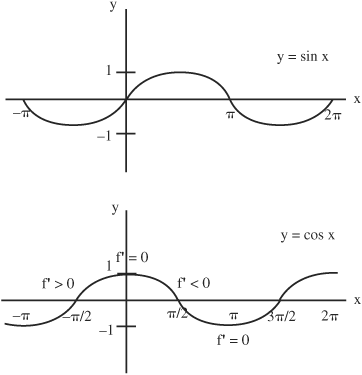
• The derivative of sine is cosine and the derivative of cosine is − sine. This can be visualized by comparing the slopes of sine and cosine curves at various points along their graphs.

The derivative of the sine curve is zero at the top and bottom points on the curve where it is horizontal, −π/2, π/2, (3/2)π, (5/2)π, etc. The maximum rates of change of sine in the positive direction occur at points on the curve at 0, 2π, 4π, etc. The maximum rates of change of the sine curve in the negative direction occur at points −π, π, 3π, etc.

The points where the derivative of sine is zero correspond to points where the cosine curve crosses zero. The points where the derivative of sine is maximum-positive correspond to maximum points on the cosine curve. Similarly, the points where the derivative on the sine curve is maximumnegative correspond to the most negative points on the cosine curve.

The cosine curve is the sine curve shifted to the left by (1/2)π, which is consistent with the trigonometric identity, cos x = sin(x + π/2)

• The derivatives of sine and cosine can be verified using the definition of the derivative and the addition formulas for sine and cosine:

sin(x+h) = sin x cos h + cos x sin h

cos(x+h) = cos x cos h − sin x sin h

For f(x) = sin x, find f′(x):

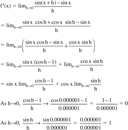
Therefore, f′(x) = 0 + cos x = cos x.

Similarly, if f(x) = cos x, find f′(x):

Therefore, f′(x) = 0 − sin x =-sin x.

• In general, the second derivative of a function indicates whether the curve is concave up (positive derivative) or concave down (negative derivative) at the point on the curve where the derivative is taken. This can be observed on the following graphs of sine and cosine.

For example at x = 0, sine begins moving up and its derivative (cosine) is positive. However, the curve is moving into a concave-down shape, which is consistent with the second derivative becoming negative.

Similarly at x = 0, cosine begins and slopes downward, its first derivative (sine) becomes negative. However, the second derivative is also negative, which is consistent with the curve moving along a concave-down shape.

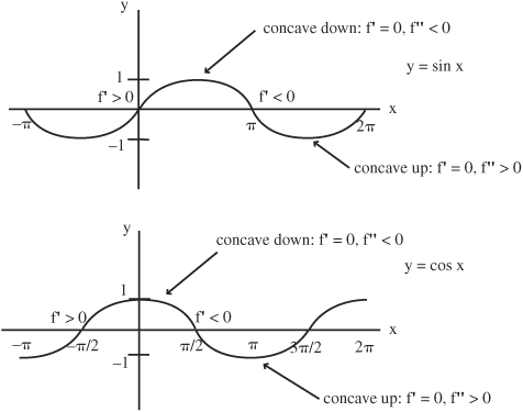
The slope at each point on the sine curve is given by the value of the cosine curve at that point.

• Second derivatives of sine and cosine are:

Tangent, Cotangent, Secant, and Cosecant

• The derivative of tangent can be easily determined using the fact that tan x = (sin x / cos x) and the rule for differentiating quotients (described in Section 2.18).

The quotient rule is

in this case, f(x) = sin x and g(x) = cos x:

(Remember, cos²x + sin²x = 1.)

• The derivatives of cotangent, secant, and cosecant are:

(d/dx)cot x = −csc²x

(d/dx)sec x = sec x tan x

(d/dx)csc x =-csc x cot x

2.22 Inverse Functions and Inverse Trigonometric Functions and Their Derivatives

• This section includes a brief summary of inverse functions, the derivative of inverse functions, inverse trigonometric functions, and their derivatives.

• Inverse functions are functions that result in the same value of x after the operations of the two functions are performed. In inverse functions, the operations of each function are the reverse of the other function. If f is the inverse of g then g is the inverse of f. Notation for the inverse of function f is f^{– 1}.

• An inverse of a function has its domain and range equal to the range and domain, respectively, of the original function. If f(x) = y, then f^–1(y) = x. For a function f(x,y) that has only one y value for each x value, then there exists an inverse function represented by f^–1(y,x). A function has an inverse if its graph intersects any horizontal line no more than once.

• If function f is represented by f(x) = u, then its inverse f^–1 can be found by solving f(x) = u for x in terms of u: f^–1u = f^–1(f(x)) = x. Therefore, if f(x) = u then f^–1(u) = x, or if f^–1(u) = x then f(x) = u. For more complicated or composite functions, if y = f[u(x)], then the inverse can be written in the opposite order: x = u^–1(f^–1(y))

• Not all functions have inverses. If a function has more than one solution, it does not have an inverse. If u(x) = z, only one x can result, x = u^–1(z). If there is more than one solution for u^–1(z), it will not be the inverse of u(x) = z.

• When functions f and u are inverse functions, then they will return to the first value. For example, if y = f(x) = 2x − 1 and x = f^-1(y) = (y + 1)/2 are inverses, and if x = 3, then by substituting for x:

f(3) = 2(3) − 1 = 5

By substituting 5 into inverse function:

f^-1(5) = (5 + 1)/2 = 3

which results in the starting point.

• Graphs of inverse functions are mirror images across the x = z line. For example, if z = u(x) = 2x, then x = (1/2)z. The slopes are (dz/dx) = 2 and (dx/dz) = 1/2.

• Following are examples of functions and their inverses:

z = x² is the inverse of: x = √z or x = z^1/2

z = e^x is the inverse of: x = ln z

z = a^x is the inverse of: x = log_az

• The derivatives of inverse functions y = f(x) and x = f^-1(y), have the property: (dy/dx)(dx/dy) = 1.

For example, using inverse functions:

y = f(x) = 2x − 1 and x = f^-1(y) = (y + 1)/2

dy/dx = 2 and dx/dy = 1/2

Therefore, (dy/dx)(dx/dy) = (2)(1/2) = 1.

• If f[u(x)] = x is an inverse function, then applying the chain rule gives: f′[u(x)] × u′(x) = 1.

If y = u(x) and x = f(y), then the rule is written:

(dx/dy)(dy/dx) = 1, where the slope of y = u(x)

multiplied by the slope of x = u^-1(y) is equal to 1.

• Inverses of trigonometric functions introduced in Chapter 1 exist in defined intervals. For example, the inverse of sine is sin^-1 y = x for 1 ≥ y ≥ −1, which pertains to sin x = y for π/2 ≥ x ≥ −π/2. The inverse brings y back to x.

The graph of y = sin x is a mirror image of sin^-1y = x.

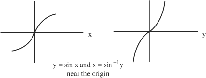
Only certain intervals of the sine function have inverses:

In the interval π/2 ≥ x −π/2, sin^-1(sin x) = x.

In the interval 1 ≥ y ≥ −1, sin(sin^-1 y) = y.

There are many points on the sine function where sin x = 0.

• The derivative of inverse sine, where x = sin^-1 y, exists in the interval 1 ≥ y ≥ −1 and π/2 ≥ x ≥ −π/2. The derivative of the inverse function equals one over the derivative of the original function. The derivative of the inverse function x = sin^-1 y can be found using the derivative of the original function y = sin x, where:

(dy/dx) = cos x

then by rearranging,

(dx/dy) = 1/cos x

Going further and using the trigonometric identity cos²x + sin²x = 1, or equivalently, cos x = (1 − sin²x)^1/2, combined with sin x = y and squaring sin² x = y²:

(dx/dy) = (d/dy)sin^-1 y = 1/cos x = 1/(1 − y²)^1/2

• The derivative of inverse cosine, where x = cos^-1 y, exists in the interval 1 ≥ y ≥ −1 and π ≥ x ≥ 0. The derivative of the inverse function x = cos^-1 y can be found using the derivative of the original function y = cos x, where:

(dy/dx) = - sin x

then by rearranging,

(dx/dy) = - 1/sin x

Going further and using the trigonometric identity cos²x + sin²x = 1, or equivalently, sin x = (1 − cos²x)^1/2, combined with cos x = y and squaring cos²x = y²:

(dx/dy) = (d/dy)cos^-1y = −1/sin x = −1/(1 − y²)^1/2

• For the tangent function tan x = y, the inverse, tan^-1 y = x exists for π/2 > x > −π/2. The derivative of inverse tangent, where x = tan^-1y, exists for ∞ > y > − ∞ and π/2 > x > −π/2. The derivative of the inverse function x = tan^-1 y can be found using the derivative of the original function y = tan x, where:

(dy/dx) =-sec²x

then by rearranging,

(dx/dy) =-1/sec²x

Going further and using the trigonometric identity sec²x = 1 + tan²x, combined with tan x = y and squaring tan²x = y²:

(dx/dy) = (d/dy)tan^-1y =-1/sec²x = 1/(1 + tan²x) = 1/(1 + y²)

• The following are derivatives of inverse cotangent, secant, and cosecant:

Derivative of cot^-1y is −1/(1 + y²),

for ∞ > y > − ∞ and π > x > 0

Derivative of sec^-1y is 1/| y | (y² − 1)^1/2,

for 1 > y > −1 and π > x > 0

Derivative of csc^-1y is −1/| y | (y² − 1)^1/2,

for 1 > y > −1 and π/2 > x > π/2

2.23 Differentiating Hyperbolic Functions

• This section includes differentiating hyperbolic functions and their inverses.

• Hyperbolic functions include sinh, cosh, tanh, coth, sech, and csch, and are introduced in Chapter 1. The properties of sine and cosine are reflected in the hyperbolic sine and cosine, sinh and cosh, respectively, such as:

(cosh x)² − (sinh x)² = 1

which is similar to:

(cos x)² + (sin x)² = 1

• Derivatives of sinh and cosh are similar to the derivatives of sine and cosine.

(d/dx)sinh x = cosh x

which is similar to:

(d/dx)sin x = cos x

(d/dx)cosh x = sinh x

which is similar to:

(d/dx)cos x = −sin x (without the“-”sign)

• The derivatives of tanh, coth, sech, and csch are:

(d/dx)tanh x = sech²x

(d/dx)coth x = −csch²x

(d/dx)sech x = −sech x tanh x

(d/dx)csch x = −csch x coth x

• Derivatives of inverse hyperbolic functions sinh^-1 x, tanh-1x, and sech-1x are:

The inverse of x = sinh y is y = sinh^-1x

(d/dx)sinh^-1x = 1/(1 + x²)^1/2

which is similar to:

(d/dx)sin^-1x = 1/(1 − x²)^1/2

The inverse of x = tanh y is y = tanh^-1x

(d/dx)tanh^-1x = 1/(1 − x²)

which is similar to:

(d/dx)tan^-1x = 1/(1 + x²)

The inverse of x = sech y is y = sech^-1x

(d/dx)sech^-1x = ±1/[x(1 − x²)^1/2]

which is similar to:

(d/dx)sec^-1x = 1/[x(1 − x²)^1/2]

• The derivatives of inverse hyperbolic functions cosh^-1x, csch_-1x, and coth_-1x are:

(d/dx)cosh^-1x = 1/(x² − 1)^1/2

d/dx)csch^-1x = ±1/[x(1 + x²)^1/2]

(d/dx)coth^-1x = 1/(1 − x²)

2.24 Differentiating Multivariable Functions

• This section introduces differentiating simple multivariable functions. See Chapter 6 for a complete discussion on differentiating multivariable functions.

• When a function that contains more than one variable is differentiated, the derivative formula can be applied to the variable that is being differentiated“with respect to,”while the other variable(s) is held constant. The variable being differentiated“with respect to,”is designated using d/dx, d/dy, d/dz, etc., for x, y, z, respectively.

• For example, differentiate the following simple functions with respect to x, y, and z:

Differentiated with respect to x.

Differentiated with respect to y.

Differentiated with respect to z.

2.25 Differentiation of Implicit Vs. Explicit Functions

• This section provides a brief explanation of implicit differentiation including two examples.

• If y is given explicitly as a function of x, it is not difficult to obtain (dy/dx) because if y = f(x), then (dy/dx) = f′(x). This is explicit differentiation. In explicit differentiation, y can be isolated and the equation can be solved for y, then differentiated. However, if y is given implicitly as a function of x, F(x,y) = 0, then the function can be differentiated as it is and then solved for dy/dx rather than attempting to isolate y first, which may not always be possible.

• For a function that cannot be solved for y first or is left in implicit form by choice, the equation can be differentiated implicitly as it is“term by term,”then solved for (dy/dx) in terms of x and y. This is called implicit differentiation.

• Example: Evaluate (dy/dx) for x⁴ + x²y³ − y⁶ + 4 = 0, which implicitly gives y as a function of x.

Taking the derivative of each term gives:

Solving for (dy/dx):

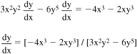
• Example: Evaluate (dy/dx) for y = e^yx + sin x, which implicitly gives y as a function of x.

Taking the derivative of each term gives:

Solving for (dy/dx):

2.26 Selected Rules of Differentiation

• This section provides a summary of selected rules of differentiation. Note that in the following functions n is a positive integer and u and v are functions of x.

2.27 Minimum, Maximum, and the First and Second Derivatives

• This section includes local and global minimum and maximum points and the first and second derivatives.

• Evaluating first and second derivatives of functions to find minimum and maximum points is a common application of the derivative. When experiments or evaluations are conducted in science, business, engineering, etc., data is gathered, relationships are developed, and graphs are constructed in order to assist in the understanding of the data and to predict future patterns and events. Information depicted in graphs, such as where the graph is rising or falling, convex or concave, or where the high and low points are located, correspond to maximum and minimum values and is crucial to the evaluation of the data.

• Consider the graph of a continuous function f:

If the highest point on f is the point (m,f(m)), then f(m) is the maximum value of f and f(m) ≥ f(x) for all x. In this graph there are two extrema points in between a and b, a minimum and a maximum where the derivative is zero.

To find the global or local extrema of a function, the graph can be inspected or the derivative can be evaluated. At the extrema points, the derivative of a function f is equal to zero. In this graph if f(n) is a minimum point and f(m) is a maximum point and if f′(n) and f′(m) exist, then f′(n) = 0 and f′(m) = 0.

• The graph of a function has a minimum or maximum point where the slope is zero and therefore the derivative is also zero, f′(x) = 0. In a region of a graph of a function where the graph is horizontal the first derivative of the function is equal to zero. A point where the graph of a function is horizontal may represent a minimum or maximum point. A minimum or maximum on the graph may be the minimum or maximum of the function, or there may be many“local”minimum or maximum points called local extrema. There can only be one global minimum and one global maximum but there may be many local extrema points.

The sign of the derivative of a function describes the shape of the graph of the function at the point where the derivative is taken.

If f(x) is decreasing as x is increasing, the sign of the derivative is negative. Therefore, f′(x) < 0 where the graph of f is decreasing.

If f(x) is increasing as x is increasing, the sign of the derivative is positive. Therefore, f′(x) > 0 where the graph of f is increasing.

If the graph of the function is horizontal, the derivative of f is zero. Therefore, f′(x) = 0 where the graph of f is horizontal.

The sign of f′(x) changes from positive to negative or negative to positive as a maximum or minimum point is crossed.

• There are examples where the graph of a function will not have a minimum or maximum, such as if the graph forms a straight horizontal or vertical line. For example:

• As a general rule, for a given function f, all values of x where f′(x) = 0 or where f′(x) is undefined, represent all possible extrema. There may, however, be cases where f′(x) = 0 but an extrema does not exist.

• By taking the second derivative of a function where the first derivative is zero, it can be determined whether the graph of that function is at a minimum and, therefore, concave up or at a maximum and, therefore, concave down. The second derivative provides information about change in slope, or the rate of change of what is changing, such as the growth rate of a population.

• If some point P is in the domain set of function f and if f′(P) exists, then the second derivative can be used to evaluate the shape of the graph as follows:

If f′(P) = 0 and if f"(P) > 0, the graph of function f is concave up at P and f has a minimum at P. Also, the slope of the curve or tangent lines drawn to the curve will begin to increase.

If f′(P) = 0 and if f"(P) < 0, the graph of function f is concave down at P and f has a maximum at P. Also, the slope of the curve or tangent lines drawn to the curve will begin to decrease.

In other words, if f′(P) exists, and if f′(P) = 0:

If f"(P) > 0 then f has a minimum at P, or

if f”(P) < 0 then f has a maximum at P.

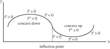
Note that in the above graph an inflection point occurs where the tangent line crosses the curve. Also, an inflection point occurs where f"(x) changes from positive to negative or negative to positive, and where the curve is concave up on one side and concave down on the other side.

• If the second derivative of a function is zero, then it does not provide information regarding whether the function is at a maximum or minimum. In this situation, information can be obtained in the region where f′(x) = 0 such that if f′(x) changes from positive to negative at f′(x) = 0, then there is a maximum at that point. Conversely, if f′(x) changes from negative to positive at f′(x) = 0, then there is a minimum at that point.

• To solve problems where minimum or maximum values need to be found, first describe the problem in terms of a function or equation, then determine f′(x) and solve for f′(x) = 0. To locate all possible extrema (minimum or maximum values of f) within some interval between x = a and x = b or between points (a,f(a)) and (b,f(b)):

(a.) Find all x values that satisfy f′(x) = 0 or f′(x) = undefined.

(b.) Evaluate each x value found in the first step by substituting it into the function f.

(c.) Evaluate values of x at the ends of the interval (at a and b) to find f(a) and f(b).

(d.) The largest value in the second step is the maximum of f(x) and the smallest value is the minimum of f(x) within the interval a-b.

(e.) Identify whether the extrema represent a minimum or maximum by determining f"(x).

• Example: Find the minimum and maximum of function f(x) = x² + 2x between the interval of x = 0 and x =-2 where −2 ≤ x ≤ 0.

First find all x values that satisfy f′(x) = 0 or f′(x) = undefined. Differentiate:

f′(x) = (d/dx)x² + (d/dx)2x = 2x + 2

Where does f′(x) = 0?

Because f′(x) = 2x + 2, set 2x + 2 = 0:

2x + 2 = 0

Solve for x:

2x =-2

x =-2/2 =-1

Evaluate each x value found by substituting it into the function f. Evaluate f(x) at x =-1.

f(-1) = x² + 2x = (-1)² + 2(-1) = 1 + −2 =-1

Evaluate the values of x at the ends of the interval (at a and b) to find f(a) and f(b).

Evaluate f(x) = x² + 2x at the end points −2 and 0.

f(-2) = (-2)² + 2(-2) = 4 + −4 = 0

f(0) = (0)² + 2(0) = 0 + 0 = 0

Therefore, the number for the critical points of f over this interval (-2 ≤ x ≤ 0) are: f(-1) = −1, f(0) = 0 and f(-2) = 0.

The largest and smallest values from the second step are the maximum of f(x) and the minimum of f(x) within the interval a-b. In this example, only f(- 1) =-1 was derived from the second step. The largest and smallest numbers computed overall are 0 and − 1, which represent the minimum and maximum points.

Plot the function f(x) = x² + 2x between the interval of x = 0 and x = −2. Select x values at and near the minimum and maximum points, and solve for f(x).

Values for x are −3, −2, −1, 0, 1, resulting in f(x) values 3, 0, −1, 0, 3.

Resulting pairs are (-3,3), (-2,0), (-1,-1), (0,0), (1,3).

Graphing the pairs is depicted as:

Therefore, f′(-1) = 0 within the interval a-b from x =-2 to x = 0, the graph of the function f(x) = x² + 2x depicts a minimum at f(- 1), and crosses zero at x =-2 and x = 0.

Evaluating the second derivative of this function, f(x) = x² + 2x, will determine whether there is a minimum or a maximum at the point where f′(x) = 0 (and therefore verify the result of the graph).

f′(x) = 2x + 2

Taking the second derivative:

f"(x) = (d/dx)2x + (d/dx)2 = 2 + 0 = 2

Using the second derivative rule, because 2 is a positive number, the graph of f(x) at x =-1 is concave up and is at a minimum. This was depicted in the graph.

2.28 Notes on Local Linearity, Approximating Slope of Curve, and Numerical Methods

• This section includes a brief introduction of local linearity and the tangent line approximation and a brief explanation of Newton’s method for equations in the form f(x) = 0.

• When calculating approximate values for complicated functions, it is sometimes possible to focus in on a small region of the graph of a function, and look at that region as if it were linear. This is sometimes referred to as a point of local linearity. In the region of a point on the graph of a function, a tangent line can be drawn and the slope of the tangent line is the derivative of the function at that point. The equation for a tangent line passing through point (a,f(a)) is: y − f(a) = f′(a)(x − a).

• The equation for the tangent line y − f(a) = f′(a)(x − a), at y = f(x) and x = a can be derived using:

f′(a) ≈ [f(a + h) − f(a)]/h

By rearranging:

f′(a)(h) ≈ f(a + h) − f(a)

f(a + h) ≈ f′(a)(h) + f(a)

Substituting x − a = h and x = a + h:

f(a + h) ≈ f′(a)(x − a) + f(a)

f(x) ≈ f′(a)(x − a) + f(a)

Substituting y = f(x):

y − f(a) = f′(a)(x − a)

This equation can be used to linearize a region of f near x = a for the tangent through (a, f(a)) for curved functions.

• For example, the tangent line approximation for f(x) = cos x, where x is near a = 0 can be calculated using:

f(x) ≈ f′(0)(x − 0) + f(0)

Substitute in for each term:

Left side term:

f(x) = cos x

The first term:

f′(0) = −sin 0 = 0

and x − 0 = x

The second term:

f(0) = cos 0 = 1

Then the equation f(x) ≈ f′(0)(x − 0) + f(0) becomes:

cos x ≈ (0)(x) + 1 = 1

cos x ≈ 1

Therefore, the tangent line approximation for

f(x) near x = 0 is y = f(x) = 1.

• Similarly for f(x) = sin x near x = 0, the tangent line approximation can be calculated using:

f(x) ≈ f′(0)(x − 0) + f(0)

Substitute in for each term:

Left side term:

f(x) = sin x

The first term:

f′(0) = cos 0 = 1

and x − 0 = x

The second term:

f(0) = sin 0 = 0

Then the equation f(x) ≈ f′(0)(x − 0) + f(0) becomes:

sin x ≈ (1)(x) + 0 = x

sin x ≈ x

Therefore, the tangent line approximation for

f(x) near x = 0 is y = f(x) = x.

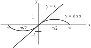
• The tangent line drawn on selected points of the graph of a function can be used in numerical differentiation methods, such as Newton’s method. Numerical methods are sometimes required to estimate and solve equations, such as finding the roots of a high-degree polynomial. In general, numerical methods can be applied to programming when a function is translated into an algorithm, solving systems of linear equations, and numerical solutions to ordinary and partial differential equations.

• The Newton method can be applied to solve equations in the form f(x) = 0 where f′(x) exists and is continuous.

In this method, the graph of f is approximated using tangent lines, thereby determining the roots (x values) of f(x). First, a value for x₀ is selected from the graph of f, then a tangent is drawn at x₀, where x₁ is the intersection of the X-axis by the tangent to the curve at x₀. This process can be repeated beginning with the value of x₁ and drawing the tangent that intercepts the X-axis at x₂. Then, repeat for x₂ to get x₃ and so on until the x’s converge.

Alternatively, after the first step the equation for a tangent line at f(x) = y, x = x₀ can be used:

y − f(x₀) = f′(x₀)(x −x₀)

where the tangent crosses the X-axis at y = 0, x = x₁, therefore:

0 − f(x₀) = f′(x₀)(x₁ − x₀)

Rearranging:

This formula can be used repeatedly for x₂, x₃, ..., x_n+1:

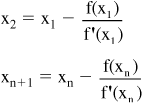
Using this formula, x_n should converge to a solution (root) of x if a solution exists. In cases where f(x) = 0 has no root or multiple roots, this formula will not converge to a single x value. Such cases include f(x) = 1 + x².