
We now have the necessary tools to learn about our first and simplest graphical model, the Naïve Bayes classifier. This is a directed graphical model that contains a single parent node and a series of child nodes representing random variables that are dependent only on this node with no dependencies between them. Here is an example:

We usually interpret our single parent node as the causal node, so in our particular example, the value of the Sentiment node will influence the value of the sad node, the fun node, and so on. As this is a Bayesian network, the local Markov property can be used to explain the core assumption of the model. Given the Sentiment node, all other nodes are independent of each other.
In practice, we use the Naïve Bayes classifier in a context where we can observe and measure the child nodes and attempt to estimate the parent node as our output. Thus, the child nodes will be the input features of our model, and the parent node will be the output variable. For example, the child nodes may represent various medical symptoms and the parent node might be whether a particular disease is present.
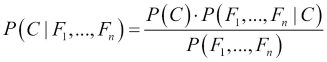
To understand how the model works in practice, we make recourse to Bayes' theorem, where C is the parent node and Fi are the children or feature nodes:
We can simplify this using the conditional independence assumptions of the network:

To make a classifier out of this probability model, our objective is to choose the class Ci which maximizes the posterior probability P(Ci|F1 …Fn ); that is, the posterior probability of that class given the observed features. The denominator is the joint probability of the observed features, which is not influenced by the class that is chosen. Consequently, maximizing the posterior class probability amounts to maximizing the numerator of the previous equation:

Given some data, we can estimate the probabilities, P(Fi |Cj ), for all the different values of the feature Fi as the relative proportion of the observations of class Cj that have each different value of feature Fi. We can also estimate P(Cj ) as the relative proportion of the observations that are assigned to class Cj. These are the maximum likelihood estimates. In the next section, we will see how the Naïve Bayes classifier works in a real example.
In a world of online reviews, forums, and social media, a task that has received, and continues to receive, a growing amount of interest is the task of sentiment analysis. Put simply, the task is to analyze a piece of text to determine the sentiment that is being expressed by the author. A typical scenario involves collecting online reviews, blog posts, or tweets and building a model that predicts whether the user is trying to express a positive or a negative feeling. Sometimes, the task can be framed to capture a wider variety of sentiments, such as a neutral sentiment or the degree of sentiment, such as mildly negative versus very negative.
In this section, we will limit ourselves to the simpler task of discerning positive from negative sentiments. We will do this by modeling sentiment using a similar Bayesian network to the one that we saw in the previous section. The sentiment is our target output variable, which is either positive or negative. Our input features are all binary features that describe whether a particular word is present in a movie review. The key idea here is that users expressing a negative sentiment will tend to choose from a characteristic set of words in their review that is different from the characteristic set that users would pick from when writing a positive review.
By using the Naïve Bayes model, our assumption will be that if we know the sentiment being expressed, the presence of each word in the text is independent from all the other words. Of course, this is a very strict assumption to use and doesn't speak at all to the process of how real text is written. Nonetheless, we will show that even under these strict assumptions, we can build a model that performs reasonably well.
We will use the Large Movie Review Data Set, first presented in the paper titled Learning Word Vectors for Sentiment Analysis, Andrew L. Maas, Raymond E. Daly, Peter T. Pham, Dan Huang, Andrew Y. Ng, and Christopher Potts, published in The 49th Annual Meeting of the Association for Computational Linguistics (ACL 2011). The data is hosted at http://ai.stanford.edu/~amaas/data/sentiment/ and is comprised of a training set of 25,000 movie reviews and a test set of another 25,000 movie reviews.
In order to demonstrate how the model works, we would like to keep the training time of our model low. For this reason, we are going to partition the original training set into a new training and test set, but the reader is very strongly encouraged to repeat the exercise with the larger test dataset that is part of the original data. When downloaded, the data is organized into a train folder and a test folder. The train folder contains a folder called pos that has 12,500 positive movie reviews, each inside a separate text file, and similarly, a folder called neg with 12,500 negative movie reviews.
Our first task is to load all this information into R and perform some necessary preprocessing. To do this, we are going to install and use the tm package, which is a specialized package for performing text-mining operations. This package is very useful when working with text data and we will use it again in a subsequent chapter.
When working with the tm package, the first task is to organize the various sources of text into a corpus. In linguistics, this commonly refers to a collection of documents. In the tm package, it is just a collection of strings representing individual sources of text, along with some metadata that describes some information about them, such as the names of the files from which they were retrieved.
With the tm package, we build a corpus using the Corpus() function, to which we must provide a source for the various documents we want to import. We could create a vector of strings and pass this as an argument to Corpus() using the VectorSource() function. Instead, as our data source is a series of text files in a directory, we will use the DirSource() function. First, we will create two string variables that will contain the absolute paths to the aforementioned neg and pos folders on our machine (this will depend on where the dataset is downloaded).
Then, we can use the Corpus() function twice to create two corpora for positive and negative reviews, which will then be merged into a single corpus:
> path_to_neg_folder <- "~/aclImdb/train/neg"
> path_to_pos_folder <- "~/aclImdb/train/pos"
> library("tm")
> nb_pos <- Corpus(DirSource(path_to_pos_folder),
                   readerControl = list(language = "en"))
> nb_neg <- Corpus(DirSource(path_to_neg_folder),
                  readerControl = list(language = "en"))
> nb_all <- c(nb_pos, nb_neg, recursive = T)
The second argument to the Corpus() function, readerControl, is a list of optional parameters. We used this to specify that the language of our text files is English. The recursive parameter in the c() function used to merge the two corpora is necessary to maintain the metadata information stored in the corpus objects.
Note that we can merge the two corpora without actually losing the sentiment label. Each text file representing a movie review is named using the format <counter>_<score>.txt, and this information is stored in the metadata portion of the corpus object created by the Corpus() function. We can see the metadata for the first review in our corpus using the meta() function:
> meta(nb_all[[1]])
Metadata:
  author       : character(0)
  datetimestamp: 2015-04-19 09:17:48
  description  : character(0)
  heading      : character(0)
  id           : 0_9.txt
  language     : en
  origin       : character(0)
The meta() function thus retrieves a metadata object for each entry in our corpus. The ID attribute in this object contains the name of the file. The score part of the name is a number between 0 and 10, where higher numbers denote positive reviews, and low numbers denote negative reviews. In the training data, we only have polar reviews; that is, reviews that are in the ranges 0-4 and 7-10. We can thus use this information to create a vector of document names:
> ids <- sapply( 1 : length(nb_all),
                 function(x) meta(nb_all[[x]], "id"))
> head(ids)
[1] "0_9.txt"     "1_7.txt"     "10_9.txt"    "100_7.txt"
[5] "1000_8.txt"  "10000_8.txt"
From this list of document names, we'll extract the score component using the sub() function with an appropriate regular expression. If the score of a movie review is less than or equal to 5, it is a negative review and if it is greater, it is a positive review:
> scores <- as.numeric(sapply(ids,
            function(x) sub("[0-9]+_([0-9]+)\.txt", "\1", x)))
> scores <- factor(ifelse(scores >= 5, "positive", "negative"))
> summary(scores)
negative positive
   12500    12500
Tip
The sub() function is just one of R's functions that uses regular expressions. For readers unfamiliar with the concept, a regular expression is essentially a pattern language for describing strings. Online tutorials for regular expressions are easy to find. An excellent resource for learning about regular expressions' as well as text processing more generally, is Speech and Language Processing Second Edition, Jurafsky and Martin.
The features of our model will be binary features that describe the presence or absence of specific words in the dictionary. Intuitively, we should expect that a movie review containing words such as boring, cliché, and horrible is likely to be a negative review. A movie review with words such as inspiring, enjoyable, moving, and excellent is likely to be a good review.
When working with text data, we almost always need to perform a series of preprocessing steps. For example, we tend to convert all the words to a lowercase format because we don't want to have two separate features for the words Excellent and excellent. We also want to remove anything from our text that will likely be uninformative as features. For this reason, we tend to remove punctuation, numbers, and stop words. Stop words are words such as the, and, in, and he, which are very frequently used in the English language and are bound to appear in nearly all of the movie reviews. Finally, because we are removing words from sentences and creating repeated spaces, we will want to remove these in order to assist the process of tokenization (the process of splitting up the text into words).
The tm package has two functions, tm_map() and content_transformer(), which together can be used to apply text transformations to the content of every entry in our corpus:
> nb_all <- tm_map(nb_all, content_transformer(removeNumbers))
> nb_all <- tm_map(nb_all, content_transformer(removePunctuation))
> nb_all <- tm_map(nb_all, content_transformer(tolower))
> nb_all <- tm_map(nb_all, content_transformer(removeWords),
                           stopwords("english"))
> nb_all <- tm_map(nb_all, content_transformer(stripWhitespace))
Now that we have preprocessed our corpus, we are ready to compute our features. Essentially, what we need is a data structure known as a document term matrix. The rows of the matrix are the documents. The columns of the matrix are the words in our dictionary. Each entry in the matrix is a binary value, with 1 representing the fact that the word represented by the column number was found inside the review represented by the row number. For example, if the first column corresponds to the word action, the fourth row corresponds to the fourth movie review, and the value of the matrix at position (4,1) is 1, this signifies that the fourth movie review contains the word action.
The tm package provides us with the DocumentTermMatrix() function that takes in a corpus object and builds a document term matrix. The particular matrix built has numerical entries that represent the total number of times a particular word is seen inside a particular text, so we will have to convert these into a binary factor afterward:
> nb_dtm <- DocumentTermMatrix(nb_all)
> dim(nb_dtm)
[1]  25000 117473
Our document term matrix in this case has 117,473 columns, indicating that we have found this number of different words in the corpus. This matrix is very sparse, meaning that most of the entries are 0. This is a very typical scenario when building document term matrices for text documents, especially text documents that are as short as movie reviews. Any particular movie review will only feature a tiny fraction of the words in the vocabulary. Let's examine our matrix to see just how sparse it is:
> nb_dtm
<<DocumentTermMatrix (documents: 25000, terms: 117473)>>
Non-/sparse entries: 2493414/2934331586
Sparsity           : 100%
Maximal term length: 64
Weighting          : term frequency (tf)
From the ratio of non-sparse to sparse entries, we can see that of the 2,936,825,000 entries in the matrix (25000 × 117473), only 2,493,414 are nonzero. At this point, we should reduce the number of columns of this matrix for two reasons. On the one hand, because the words in our vocabulary will become the features in our model, we don't want to build a model that uses 117,473 features. This would take a very long time to train and, at the same time, is unlikely to provide us with a decent fit using only 25,000 data points.
Another significant reason for us to want to reduce the number of columns is that many words will appear only once or twice in the whole corpus, and will be as uninformative about the user's sentiment as words that occur in nearly all the documents. Given this, we have a natural way to reduce the dimensions of the document term matrix, namely by dropping the columns (that is, removing certain words from the feature set) that are the sparsest. We can remove all columns that have a certain percentage of sparse elements using the removeSparseTerms() function. The first argument that we must provide this with is a document term matrix, and the second is the maximum degree of column sparseness that we will allow. Choosing the degree of sparseness is tricky because we don't want to throw away too many of the columns that will become our features. We will proceed by running our experiments with 99 percent sparseness, but encourage the reader to repeat with different values to see the effect this has on the number of features and model performance.
We have 25,000 rows in the matrix corresponding to the total number of documents in our corpus. If we allow a maximum of 99 percent sparseness, we are effectively removing words that do not occur in at least 1 percent of those 25,000 documents; that is, in at least 250 documents:
> nb_dtm <- removeSparseTerms(x = nb_dtm, sparse = 0.99)
> dim(nb_dtm)
[1] 25000  1603
We have now significantly reduced the number of columns down to 1,603. This is a substantially more reasonable number of features for us to work with. Next, we convert all entries to binary, using another function of tm, weightBin():
> nb_dtm <- weightBin(nb_dtm)
As the document term matrix is, in general, a very sparse matrix, R uses a compact data structure to store the information. To peek inside this matrix and examine the first few terms, we will use the inspect() function on a small slice of this matrix:
> inspect(nb_dtm[10:16, 1:6])
<<DocumentTermMatrix (documents: 7, terms: 6)>>
Non-/sparse entries: 2/40
Sparsity           : 95%
Maximal term length: 10
Weighting          : binary (bin)
             Terms
Docs          ability able absolute absolutely absurd academy
  10004_8.txt       0    1        0          0      0       0
  10005_7.txt       0    0        0          0      0       0
  10006_7.txt       0    0        0          0      0       0
  10007_7.txt       0    0        0          0      0       0
  10008_7.txt       0    0        0          0      0       1
  10009_9.txt       0    0        0          0      0       0
  1001_8.txt        0    0        0          0      0       0
It looks like the word ability does not appear in the first six documents and the word able appears in the document 10004_8.txt. We now have both our features and our output vector. The next step is to convert our document term matrix into a data frame. This is needed by the function that will train our Naïve Bayes model. Then, before we train the model, we will split our data into a training set with 80 percent of the documents and a test set with 20 percent of the documents, as follows:
> nb_df <- as.data.frame(as.matrix(nb_dtm))
> library(caret)
> set.seed(443452342)
> nb_sampling_vector <- createDataPartition(scores, p = 0.80,
                                            list = FALSE)
> nb_df_train <- nb_df[nb_sampling_vector,]
> nb_df_test <- nb_df[-nb_sampling_vector,]
> scores_train = scores[nb_sampling_vector]
> scores_test = scores[-nb_sampling_vector]
To train a Naïve Bayes model, we will use the naiveBayes() function in the e1071 package that we saw earlier. The first argument we will provide it with is our feature data frame, and the second argument is our vector of output labels:
> library("e1071")
> nb_model <- naiveBayes(nb_dtm_train, scores_train)
We can use the predict() function to obtain predictions on our training data:
> nb_train_predictions <- predict(nb_model, nb_df_train)
> mean(nb_train_predictions == scores_train)
[1] 0.83015
> table(actual = scores_train, predictions = nb_train_predictions)
          predictions
actual     negative positive
  negative     8442     1558
  positive     1839     8161
We have hit over 83 percent training accuracy with our simple Naïve Bayes model, which, admittedly, is not bad for such a simple model with an independence assumption that we know is not realistic for our data. Let's repeat the same on our test data:
> nb_test_predictions <- predict(nb_model, nb_df_test)
> mean(nb_test_predictions == scores_test)
[1] 0.8224
> table(actual = scores_test, predictions = nb_test_predictions)
          predictions
actual     negative positive
  negative     2090      410
  positive      478     2022
The test accuracy of over 82 percent is comparable to what we saw on our training data. There are a number of potential avenues for improvement here. The first involves noticing that words such as movie and movies are treated differently, even though they are the same word but inflected. In linguistics, inflection is the process by which the base form or lemma of a word is modified to agree with another word on attributes such as tense, case, gender, and number. For example, in English, verbs must agree with their subject.
The tm package supports stemming, a process of removing the inflected part of a word in order to keep just a stem or root word. This is not always the same as retrieving what is known as the morphological lemma of a word, which is what we look up in a dictionary, but is a rough approximation. The tm package uses the well-known Porter Stemmer.
Note
Martin Porter, the author of the Porter Stemmer, maintains a website at http://tartarus.org/martin/PorterStemmer/, which is a great source of information on his famous algorithm.
To apply stemming to our corpus, we need to add a final transformation to our corpus using tm_map() and then recompute our document term matrix anew, as the columns (the word features) are now word stems:
> nb_all <- tm_map(nb_all, stemDocument, language = "english")
> nb_dtm <- DocumentTermMatrix(nb_all)
> nb_dtm <- removeSparseTerms(x = nb_dtm, sparse = 0.99)
> nb_dtm <- weightBin(nb_dtm)
> nb_df_train <- nb_df[nb_sampling_vector,]
> nb_df_test <- nb_df[-nb_sampling_vector,]
> dim(nb_dtm)
[1] 25000  1553
Note that we have fewer columns that match our criterion of 99 percent maximum sparsity. We can use this new document term matrix to train another Naïve Bayes classifier and then measure the accuracy on our test set:
> nb_model_stem <- naiveBayes(nb_df_train, scores_train)
> nb_test_predictions_stem <- predict(nb_model_stem, nb_df_test)
> mean(nb_test_predictions_stem == scores_test)
[1] 0.8
> table(actual = scores_test, predictions =
                              nb_test_predictions_stem)
          predictions
actual     negative positive
  negative     2067      433
  positive      567     1933
The result, 80 percent, is slightly lower than what we observed without stemming, although we are using slightly fewer features than before. Stemming is not always guaranteed to be a good idea, as in some problems it may improve performance, whereas in others it will make no difference or even make things worse. It is, however, a common transformation that is worth trying when working with text data.
A second possible improvement is to use additive smoothing (also known as laplacian smoothing) during the training of our Naïve Bayes model. This is actually a form of regularization and it works by adding a fixed number to all the counts of feature and class combinations during training. Using our original document term matrix, we can compute a Naïve Bayes model with additive smoothing by specifying the laplace parameter. For our particular dataset, however, we did not witness any improvements by doing this.
There are a few more avenues of approach that we might try with a Naïve Bayes model, and we will propose them here for the reader to experiment with. The first of these is that it is often worth manually curating the list of words used as features for the model. When we study the terms selected by our document term matrix, we may find that some words are frequent in our training data, but we do not expect them to be frequent in general, or representative of the overall population. Furthermore, we may only want to experiment with words that we know are suggestive of emotion and sentiment. This can be done by specifying a specific dictionary of terms to use when constructing our document term matrix. Here is an example:
> emotion_words <- c("good", "bad", "enjoyed", "hated", "like")
> nb_dtm <- DocumentTermMatrix(nb_all, list(dictionary =
                                            emotion_words))
It is relatively straightforward to find examples of such lists on the internet. Another common preprocessing step that is used with a Naïve Bayes model is to remove correlations between features. One way of doing this is to perform PCA, as we saw in Chapter 1, Gearing Up for Predictive Modeling. Furthermore, this method also allows us to begin with a slightly more sparse document term matrix with a larger number of terms, as we know we will be reducing the overall number of features with PCA.
Potential model improvements notwithstanding, it is important to be aware of the limitations that the Naïve Bayes model imposes that impede our ability to train a highly accurate sentiment analyzer. Assuming that all the words in a movie review are independent of each other, once we know the sentiment involved, is quite an unrealistic assumption. Our model completely disregards sentence structure and word order. For example, the phrase not bad in a review might indicate a positive sentiment, but because we look at words in isolation, we will tend to correlate the word bad with a negative sentiment.
Negation in general is one of the hardest problems to handle in text processing. Our model also cannot handle common patterns of language, such as sarcasm, irony, quoted passages that include other people's thoughts, and other such linguistic devices.
The next section will introduce a more powerful graphical model.
Note
Hidden Markov models
A good reference to study for the Naïve Bayes classifier is An empirical study of the Naïve Bayes classifier, I. Rish, presented in the 2001 IJCAI workshop on Empirical Methods in AI. For sentiment analysis, we recommend the slides from Bing Liu's AAAI 2011 tutorial at (as of this writing) https://www.researchgate.net/profile/Irina_Rish/publication/228845263_An_Empirical_Study_of_the_Naive_Bayes_Classifier/links/00b7d52dc3ccd8d692000000/An-Empirical-Study-of-the-Naive-Bayes-Classifier.pdf.
A Hidden Markov model, often abbreviated to HMM, which we will use here, is a Bayesian network with a repeating structure that is commonly used to model and predict sequences. In this section, we'll see two applications of this model: one to model DNA gene sequences, and another to model the sequences of letters that make up English text. The basic diagram for an HMM is shown here:

As we can see in the diagram, the sequence flows from left to right and we have a pair of nodes for every entry in the sequence that we are trying to model. Nodes labeled Ci are known as latent states, hidden states, or merely states, as they are typically nodes that are not observable. The nodes labeled Oi are observed states or observations. We will use the terms states and observations.
Now, as this is a Bayesian network, we can immediately identify some key properties. All the observations are independent of each other given their corresponding state. Also, every state is independent of every other state earlier on in the sequence history, given the state that preceded it (which is its parent in the network). The key idea behind an HMM, therefore, is that the model moves in a linear fashion from one state to the next state.
In each latent state, it produces an observation, which is also known as an emitted symbol. These symbols are the observed part of the sequence. Hidden Markov models are very common in natural language processing, and a good example is their application to part of speech tagging. The task of a part of speech tagger is to read a sentence and return the sequence of corresponding part of speech labels for the words in that sentence. For example, given the previous sentence, a part of speech tagger might return determiner for the word The, singular noun for the word task, and so on.
To model this using an HMM, we would have the words be the emitted symbols, and the part of speech tags be the latent states, as the former are observable and the latter are what we want to determine. There are many other sequence labeling tasks in natural language processing to which Hidden Markov models have been applied, such as named entity recognition, where the goal is to identify the words in a sentence that refer to names of individuals, locations, organizations, and other entities.
A Hidden Markov model is comprised of five core components. The first of these is the set of possible latent class labels. For the part of speech tagger example, this might be a list of all the part of speech tags that we will use. The second component is the set of all possible emitted symbols. For an English part of speech tagger, this is the dictionary of English words.
The next three components involve probabilities. The starting probability vector is a vector of probabilities that tells us the probability of starting in each latent state. For part of speech tagging, we may, for example, have a high probability of starting with a determiner such as the. The transition probability matrix is a matrix that tells us the probability of going to state Cj when the current state is Ci. Thus, this contains the probability of moving from a determiner to a noun for our part of speech example. Finally, the emission probability matrix tells us the probability of emitting every symbol in our dictionary for every state that we can be in. Note that some words (such as bank, which is both a noun and a verb) can be labeled with more than one part of speech tag, and so will have nonzero probabilities of being emitted from more than one state.
In circumstances such as part of speech tagging, we usually have a collection of labeled sequences so that our data contains both sequences of observations as well as their corresponding states. In this case, similar to the Naïve Bayes model, we use relative frequency counts to populate the probability components of our model.
For example, to find a suitable starting probability vector, we could tabulate the starting state for every sequence in our dataset and use this to get the relative frequency of beginning in each state. When all we have are unlabeled sequences, the task is significantly harder because we might not even know how many states we need to include in our model. One method to assign states to unlabeled observation sequences in training data is known as the Baum-Welch algorithm.
Once we know the parameters of our model, the question becomes how to predict the most likely sequence of states behind a sequence of observations. Given an unlabeled sentence in English, a part of speech tagger based on an HMM must predict the sequence of part of speech labels. The most commonly used algorithm for this is based on a programming technique known as dynamic programming and is known as the Viterbi algorithm.
The algorithms we have discussed for the Hidden Markov model are beyond the scope of this book, but are quite intuitive and well worth studying. Given a basic understanding of the core components of the model and its assumptions, our next goal is to see how we can apply them to some real-world situations. We will first see an example with labeled sequences and later, an example with unlabeled sequences.
Tip
Perhaps the most definitive and thorough introduction to Hidden Markov models is the seminal paper titled A Tutorial on Hidden Markov Models and Selected Applications in Speech Recognition, L. R. Rabiner, published in the Proceedings of the IEEE, 1989. The Jurafsky and Martin textbook we mentioned earlier is also an ideal reference to learn more about HMMs, including details on the Baum-Welch and Viterbi algorithms, as well as applications such as part of speech tagging and named entity recognition.
The first application we will study in detail comes from the field of biology. There, we learn that the basic building blocks of DNA molecules are actually four fundamental molecules known as nucleotides. These are called Thymine, Cytosine, Adenine, and Guanine, and it is the order in which these molecules appear in a DNA strand that encodes the genetic information carried by the DNA.
An interesting problem in molecular biology is finding promoter sequences within a larger DNA strand. These are special sequences of nucleotides that play an important role in regulating a genetic process known as gene transcription. This is the first step in the mechanism by which information in the DNA is read.
The molecular biology (promoter gene sequences) dataset, hosted by the UCI Machine Learning repository at https://archive.ics.uci.edu/ml/datasets/Molecular+Biology+(Promoter+Gene+Sequences), contains a number of gene sequences from DNA belonging to the bacterium E. Coli.
The predictive task at hand is to build a model that will discern promoter gene sequences from non-promoter gene sequences. We will approach this problem using HMMs. Specifically, we will build an HMM for promoters and an HMM for non-promoters, and we will pick the model that gives us the highest probability for a test sequence in order to label that sequence:
> promoters <- read.csv("promoters.data", header = F, dec = ",",
               strip.white = TRUE, stringsAsFactors = FALSE)
> promoters[1,]
  V1  V2                                                        V3
1  + S10 tactagcaatacgcttgcgttcggtggttaagtatgtataatgcgcgggcttgtcgt
Note that it is important to strip whitespace using the strip.white = TRUE parameter setting in the call to read.csv(), as some fields have leading tab characters. The first column in the data frame contains a + or - to denote promoters or non-promoters respectively. The second column is just an identifier for the particular sequence and the third column is the sequence of nucleotides itself. We'll begin by separating the data into positive and negative observations of promoter sequences using the first column:
> positive_observations <- subset(promoters, V1 == '+', 3)
> negative_observations <- subset(promoters, V1 == '-', 3)
In order to train our HMMs, we want to concatenate all the observations from each class into a single observation. We do, however, want to store information about the start and end of each sequence. Consequently, we will prepend each sequence with the character S to denote the start of a sequence and append each sequence with the character X to denote the end of a sequence:
> positive_observations <- sapply(positive_observations,
                           function(x) paste("S", x, "X", sep=""))
> negative_observations <- sapply(negative_observations,
                           function(x) paste("S", x, "X", sep=""))
> positive_observations[1]
[1] "StactagcaatacgcttgcgttcggtggttaagtatgtataatgcgcgggcttgtcgtX"
Next, we will split each observation from a string into a vector of characters using the strsplit() function, which takes a string to split as the first argument and the character to use as the split points (delimiter). Here, we use an empty character on which to split, so that the whole string is broken up into single characters:
> positive_observations <- strsplit(positive_observations, "")
> negative_observations <- strsplit(negative_observations, "")
> head(positive_observations[[1]], n = 15)
 [1] "S" "t" "a" "c" "t" "a" "g" "c" "a" "a" "t" "a" "c" "g" "c"
Now we have to specify the probability matrices for the HMMs that we want to train. In this particular situation, the states have a one-to-one correspondence with the emitted symbols, so in fact this type of problem can be simplified to a visible Markov model, which in this case is just a Markov chain. Nonetheless, the process we will follow for modeling this problem as an HMM is the same that we would follow in the more general case of having multiple symbols assigned to each state. We are going to assume that both positive and negative HMMs involve four states corresponding to the four nucleotides. Although both models will emit the same symbols in each state, they will differ in their transition probabilities from one state to the next.
Apart from the four states we mentioned earlier, we created a special terminating state at the end of each sequence using the symbol X. We also created a special starting state, which we called S, so that the starting probability of all the other states is 0. In addition, the emission probabilities are trivial to compute as only one symbol is emitted per state. Due to the one-to-one correspondence between states and symbols, we will use the same alphabet to represent the states and the symbols they emit:
> states <- c("S", "X", "a", "c", "g", "t")
> symbols <- c("S", "X", "a", "c", "g", "t")
> startingProbabilities <- c(1,0,0,0,0,0)
> emissionProbabilities <- diag(6)
> colnames(emissionProbabilities) <- states
> rownames(emissionProbabilities) <- symbols
> emissionProbabilities
  S X a c g t
S 1 0 0 0 0 0
X 0 1 0 0 0 0
a 0 0 1 0 0 0
c 0 0 0 1 0 0
g 0 0 0 0 1 0
t 0 0 0 0 0 1
Computing the transition probability matrix requires us to do a bit more work. Thus, we defined our own function for this: calculateTransitionProbabilities(). The input to this function is a single vector of training sequences concatenated with each other, along with a vector containing the names of the states.
The function first computes an empty transition probability matrix. By cycling over each consecutive pair of states, it tallies up counts of state transitions. After all the data has been traversed, we normalize the transition probability matrix by dividing each row of the matrix by the sum of the elements in that row. This is done because the rows of this matrix must sum to one. We use the sweep() function, which allows us to apply a function on every element of the matrix using a summary statistic. Here is calculateTransitionProbabilities():
calculateTransitionProbabilities <- function(data, states) {
  transitionProbabilities <- matrix(0, length(states), length(states))
  colnames(transitionProbabilities) <- states
  rownames(transitionProbabilities) <- states
  for (index in 1:(length(data) - 1)) {
    current_state <- data[index]
    next_state <- data[index + 1]
    transitionProbabilities[current_state, next_state] <-
           transitionProbabilities[current_state, next_state] + 1
  }
  transitionProbabilities <- sweep(transitionProbabilities, 1,
           rowSums(transitionProbabilities), FUN = "/")
  return(transitionProbabilities)
}
Now we are ready to train our models. The key observation to make on this dataset is that we have very few observations, just 53 of each class in fact. This dataset is too small to set a portion aside for testing. Instead, we will implement leave-one-out cross validation to estimate the accuracy of our models. To do this, we will begin by leaving an observation out from the positive observations. This leaves all the negative observations available for computing the transition probability matrix for our negative HMM:
> negative_observation<-Reduce(function(x, y) c(x, y),
                               negative_observations, c())
> (transitionProbabilitiesNeg <-
   calculateTransitionProbabilities(negative_observation, states))
  S          X         a         c         g         t
S 0 0.00000000 0.2264151 0.2830189 0.1320755 0.3584906
X 1 0.00000000 0.0000000 0.0000000 0.0000000 0.0000000
a 0 0.02168022 0.2113821 0.2696477 0.2506775 0.2466125
c 0 0.01256983 0.2500000 0.1634078 0.2667598 0.3072626
g 0 0.01958225 0.3133159 0.2480418 0.1919060 0.2271540
t 0 0.01622971 0.1885144 0.2434457 0.2946317 0.2571785
When in the start state (S), we can randomly move to a nucleotide state, but have zero probability of moving to the stop state (X) or staying in the start state. When in the nucleotide states, we can randomly transition to any state except back to the start state. Finally, the only valid transition from a stop state is to the start state for a new sequence.
We now introduce the HMM package in R, which is for working with Hidden Markov models, as the name implies. We can initialize an HMM with a specific set of parameters using the initHMM() function. As expected, this takes five inputs corresponding to the five components of a Hidden Markov model, which we discussed earlier:
> library("HMM")
> negative_hmm <- initHMM(states, symbols, startProbs =
  startingProbabilities, transProbs = transitionProbabilitiesNeg,
  emissionProbs = emissionProbabilities)
The next step is to build the positive HMM, but we will have to do this multiple times, leaving out one observation for testing. This test observation will then be processed by the negative HMM we trained earlier and the positive HMM that was trained without that observation. If the positive HMM predicts a higher probability for the test observation than the negative HMM, our model will correctly classify the test observation. The following block of code performs a loop of these calculations for every positive observation:
> incorrect <- 0
> for (obs in 1 : length(positive_observations)) {
     positive_observation <- Reduce(function(x, y) c(x, y),
                             positive_observations[-obs], c())
     transitionProbabilitiesPos  <-
    calculateTransitionProbabilities(positive_observation, states)
     positive_hmm <- initHMM(states, symbols,
                          startProbs = startingProbabilities,
                          transProbs = transitionProbabilitiesPos,
                          emissionProbs = emissionProbabilities)
     test_observation <- positive_observations[[obs]]
     final_index <- length(test_observation)
     pos_probs <- exp(forward(positive_hmm, test_observation))
     neg_probs <- exp(forward(negative_hmm, test_observation))
     pos_seq_prob <- sum(pos_probs[, final_index])
     neg_seq_prob <- sum(neg_probs[, final_index])
     if (pos_seq_prob < neg_seq_prob) incorrect <- incorrect + 1
 }
We'll now walk through the previous code block. Firstly, we keep track of any mistakes we make using the incorrect variable. For every observation in our positive observations list, we'll train a positive HMM without this observation. This observation then becomes our test observation.
To find the probability of a particular sequence given a particular HMM, we used the forward() function, which computes a matrix containing the logarithm of all the forward probabilities for every step in the observation sequence. The final column in this matrix, whose numerical index is just the length of the sequence, contains the forward probability for the whole sequence. We compute the positive sequence probability using the positive HMM that we trained and use the exp() function to undo the logarithm operation (although not strictly necessary in this case, where we just need a comparison). We repeat this for the negative sequence probability using the negative HMM. As our test observation was one of the positive observations, we will misclassify only if the negative sequence probability is greater than the positive sequence probability. After our code block completes its execution, we can see how many mistakes we have made:
> incorrect
[1] 13
This means that out of the 53 positive observations, we misclassified 13 and correctly classified 40. We are not done yet, though, as we need to do a similar loop with the negative observations. This time, we will train a positive HMM once with all the positive observations:
> positive_observation <- Reduce(function(x, y) c(x, y),
                                 positive_observations, c())
> transitionProbabilitiesPos  <-
  calculateTransitionProbabilities(positive_observation, states)
> positive_hmm = initHMM(states, symbols, startProbs =
  startingProbabilities, transProbs = transitionProbabilitiesPos,
  emissionProbs = emissionProbabilities)
Next, we are going to iterate over all the negative observations. We will train a negative model by leaving one observation out as the test observation. We will then process this observation with both the positive HMM we just trained and the negative HMM trained without this observation in its training data.
Finally, we will compare the predicted sequence probability for this test observation produced by the two HMMs and classify the test observation according to which model produced the higher probability. In essence, we are doing exactly the same process as we did earlier when we were iterating over the positive observations. The following code block will continue to update our incorrect variable and should be self-explanatory:
> for (obs in 1:length(negative_observations)) {
     negative_observation<-Reduce(function(x, y) c(x, y),
                           negative_observations[-obs], c())
     transitionProbabilitiesNeg <-
    calculateTransitionProbabilities(negative_observation, states)
     negative_hmm <- initHMM(states, symbols,
                         startProbs = startingProbabilities,
                         transProbs = transitionProbabilitiesNeg,
                         emissionProbs = emissionProbabilities)
     test_observation <- negative_observations[[obs]]
     final_index <- length(test_observation)
     pos_probs <- exp(forward(positive_hmm,test_observation))
     neg_probs <- exp(forward(negative_hmm,test_observation))
     pos_seq_prob <- sum(pos_probs[, final_index])
     neg_seq_prob <- sum(neg_probs[, final_index])
     if (pos_seq_prob > neg_seq_prob) incorrect <- incorrect+1
 }
The overall number of misclassifications in the cross-validation is stored in the incorrect variable:
> incorrect
[1] 25
> (cross_validation_accuracy <- 1 - (incorrect/nrow(promoters)))
 [1] 0.7641509
Our overall cross-validation accuracy is roughly 76 percent. Given that we are using the leave-one-out approach, and that the overall size of the training data is so small, we expect this estimate to have a relatively high variance.
In our HMM, the Markov property essentially makes the assumption that only the previous nucleotide determines the choice of the next nucleotide in the sequence. We can reasonably expect that there are longer-range dependencies at work and, as a result, we are limited in accuracy by the assumptions of our model. For this reason, there are models, such as the Trigram HMM, that take into account additional states in the past other than the current state.
In the next section, we will study an example where we train a Hidden Markov model using unlabeled data. We will manually define the number of hidden states and use the Baum-Welch algorithm to train an HMM while estimating both state transitions and emissions.
In this section, we will model the patterns of letters that form English words. Beyond having different words, and sometimes alphabets, languages differ from each other in the patterns of letters that are used to form words. English words have a characteristic distribution of letters and letter sequences and, in this section, we will try to model the process of word formation in a very simplistic way by using a Hidden Markov model.
The emitted symbols of our model will be the letters themselves but this time, we don't know what the states could be as we are using unlabeled data. For this reason, we are going to provide just the number of states that we want our model to have, and then use the Baum-Welch algorithm to train the parameters of our HMM.
All we need for this task is a corpus of text in English. Earlier in this chapter, we studied movie reviews with the Naïve Bayes classifier, so we will use these for convenience, although other sources of English text could be used as well. We shall begin by reloading our movie reviews and will use the tm package to transform them all to lowercase:
> library("tm")
> nb_pos <- Corpus(DirSource(path_to_pos_folder),
                   readerControl = list(language = "en"))
> nb_neg <- Corpus(DirSource(path_to_neg_folder),
                  readerControl = list(language = "en"))
> nb_all <- c(nb_pos, nb_neg, recursive = T)
> nb_all <- tm_map(nb_all, content_transformer(tolower))
Next, we will read the text from every review and collect these in a single vector:
> texts <- sapply(1 : length(nb_all), function(x) nb_all[[x]])
To simplify our task, aside from the individual letters, we will consider a category with all the whitespace characters (spaces, tabs, and so on) and represent these with the uppercase letter W. We will do the same for numerical digits with the uppercase character N, all punctuation marks with the uppercase character P, and use the uppercase character O for anything that is left. We use regular expressions for this:
> texts <- sapply(texts, function(x) gsub("\s", "W", x))
> texts <- sapply(texts, function(x) gsub("[0-9]", "N", x))
> texts <- sapply(texts, function(x) gsub("[[:punct:]]", "P", x))
> texts <- sapply(texts, function(x) gsub("[^a-zWNP]", "O", x))
Once we have transformed all our text, we'll pick out a sample and split each review into characters. The sequences of characters from each review will then be concatenated with each other to create one long character sequence. This works quite well in this context as the corpus of reviews contains complete sentences and concatenating them amounts to joining up complete sentences. We've chosen to use a sample of 100 movie reviews. We can use more, but the time taken to train the model would be longer:
> big_text_splits <- lapply(texts[1:100],
                            function(x) strsplit(x, ""))
> big_text_splits <- unlist(big_text_splits, use.names = F)
Next, we'll want to initialize our HMM. In this example, we'll consider a model with three states, which we'll arbitrarily name s1, s2, and s3. For emitted symbols, we have the lowercase alphabet and the four uppercase characters that, as we saw earlier, are being used to represent four special character categories such as numbers. R holds a vector of lowercase letters in the variable letters, which is very convenient for us:
> states <- c("s1", "s2", "s3")
> numstates <- length(states)
> symbols <- c(letters, "W", "N", "P", "O")
> numsymbols <- length(symbols)
Next, we'll create random starting, emission, and transmission probability matrices. We'll generate random entries in the [0,1] interval using the runif() function. We will need to normalize every row in these matrices in order to ensure that the entries correspond to probabilities. To achieve this, we'll use the sweep() function as we did earlier:
> set.seed(124124)
> startingProbabilities <- matrix(runif(numstates), 1, numstates)
> startingProbabilities <- sweep(startingProbabilities, 1,
                           rowSums(startingProbabilities), FUN = "/")
> set.seed(454235)
> transitionProbabilities <- matrix(runif(numstates * numstates),
                      numstates, numstates)
> transitionProbabilities <- sweep(transitionProbabilities, 1,
                      rowSums(transitionProbabilities), FUN = "/")
> set.seed(923501)
> emissionProbabilities <- matrix(runif(numstates * numsymbols),
                      numstates, numsymbols)
> emissionProbabilities <- sweep(emissionProbabilities, 1,
                      rowSums(emissionProbabilities), FUN = "/")
We now initialize and train the HMM using the large character sequence we obtained earlier. This will take several minutes to run depending on the computational resources available, and this is the main reason we drew only a sample of the text earlier on:
> hmm <- initHMM(states, symbols,  startProbs =
      startingProbabilities, transProbs = transitionProbabilities,
      emissionProbs = emissionProbabilities)
> hmm_trained <- baumWelch(hmm, big_text_splits)
We trained our model in a completely unsupervised way by simply providing it with character sequences. We don't have a meaningful test dataset on which to assess the performance of our model; rather, this exercise is worthwhile in that it produces an HMM that has interesting properties. It is instructive to take a peek at the symbol emission probabilities for each state. These are accessible via the hmm$emissionProbs attribute on the hmm_trained object:

Let's examine these states carefully. All states have a relatively high probability of emitting a whitespace character. State 3 is very interesting as, besides whitespace, it seems to have grouped together punctuation and vowels. The HMM has successfully managed to group together the letters a, e, i, o, and u in the same category without any prior information about the English language.
This state also emits two consonants with a noticeable probability. The consonant y is emitted, which we know occasionally does behave like a vowel in words such as rhythm and phylum, for example. The consonant s is also emitted, and because it is often used to form the plural of nouns, we find this at the end of words just like punctuation marks. So, we see that this state seems to have grouped two main themes.
By contrast, state 1 tends to emit consonants and not vowels. In fact, only the vowel u seems to have a small probability of being emitted from this state. State 2 has a mix of vowels and consonants, but it is the only state in which the consonant h has a high probability. This is very interesting, as h is another letter of the alphabet that has vowel-like properties in pronunciation (it is often silent or part of a diphthong). We can learn more by examining the transition probabilities between the states:
> (trained_transition_probabilities <- hmm_trained$hmm$transProbs)
    to
from           s1           s2         s3
  s1 1.244568e-01 5.115204e-01 0.36402279
  s2 7.739387e-05 2.766151e-01 0.72330746
  s3 9.516911e-01 5.377194e-06 0.04830349
Again, we can discover a wealth of interesting properties. For example, when we are in state 3, the vowel state, we have a 95 percent chance of going to state 1, the consonant state. This is quite intuitive, in that English rarely has consecutive vowels. When we are in state 1, we have a 36 percent chance of going to the vowel state and a 51 percent chance of going to state 2.
Now we can begin to understand what state 2 represents. It primarily represents the state that emits the second consonant when we have two consecutive consonants. This is why the letter h has such a high probability in this state, as it participates in very common diphthongs, such as ch, sh, and th, the latter of course being found in very frequent words such as the. From this state, the most common successor state, with 72 percent probability, is the vowel state, as expected after two consecutive consonants.
This experiment is worth repeating with different conditions. If we use different seeds or sample a different number of movie reviews, we may see different results, as the Baum-Welch algorithm is sensitive to initial conditions and is unsupervised. Specifically, our Hidden Markov model might learn a completely different set of states.
For example, on some iterations, we noticed that all punctuation and numerical digits are grouped into one state, another state becomes the vowel state, and the third state is a pure consonant state. We can reproduce this behavior if, in the previous code, we sample 40 texts and use the numbers 1816, 1817, and 1818 for the three seeds. There are many more possibilities—some of which are easier to interpret than others.
Another parameter that is worth varying here is the number of states. If we use two states, then the split tends to be between vowels and consonants. If we increase the number of states, we will often continue to find results that are interpretable for as many as 10 states. Hidden Markov models are often also referred to as generative models because we can use them to generate examples of states and observations once they have been trained. We can do this with the simHMM() function by providing our model and the length of the sequence we want to generate:
> set.seed(987987)
> simHMM(hmm_trained$hmm, 30)
$states
 [1] "s2" "s3" "s1" "s3" "s3" "s1" "s3" "s3" "s1" "s1" "s2" "s3"
[13] "s3" "s1" "s2" "s3" "s1" "s2" "s2" "s2" "s3" "s1" "s2" "s2"
[25] "s3" "s1" "s2" "s3" "s1" "s2"
$observation
 [1] "h" "o" "P" "P" "a" "n" "W" "i" "r" "r" "h" "e" "i" "n" "h"
[16] "o" "n" "l" "W" "h" "e" "s" "t" "W" "e" "t" "c" "e" "P" "W"
As a final point, we can download and use the markovchain package, take our learned transition probability matrix, and find out in the long run how much time our model spends in each state. This is done using a steady state calculation, the mathematics of which we will not explore in this book. Thankfully, the markovchain package has a simple way to initialize a Markov chain when we know the probabilities that are involved. It does this by using the simpleMc() function, and we can use the steadyStates() function on our Markov chain to find out the steady state distribution:
> library("markovchain")
> simpleMc<-new("markovchain", states = c("s1", "s2", "s3"),
                transitionMatrix = trained_transition_probabilities,
                name = "simpleMc")
> steadyStates(simpleMc)
            s1       s2        s3
[1,] 0.3806541 0.269171 0.3501748
In the long term, we spend 38 percent of our time in state 1, the first consonant state; 27 percent in state 2, the second consonant state; and 35 percent of our time in state 3, the main vowel state.