
Financial and economic models primarily help in the simplification and abstraction of data and make extensive use of probability and statistics. It's always important to take a look at the data; the first step in data analysis should be plotting the data. Problems such as bad data, outliers, and missing data can often be detected by visualizing data. Bad data should be corrected whenever possible or otherwise discarded. However, in some unusual cases, such as in a stock market, outliers are good data and should be retained. To summarize, it is important to detect the bad data and outliers and to understand them so that appropriate action can be taken. The choice of data variables plays an important role in these models.
The selection of variables is important because the nature of a model will often determine the facts that are being looked at. For instance, in order to measure inflation, a model of behavior is required so that you can understand the real changes in price, and the changes in price that directly connect to inflation.
There are many interesting models and their applications that we can discuss, but to stay within the scope of this book, we will select some examples. In some cases, such as Monte Carlo, we will also select some application in sports. In the later sections, we will discuss the following topics:
- Monte Carlo simulation—examples applicable in many areas
- Price models with examples
- Understanding volatility measures with examples
- The threshold model—Shelling's model of segregation
- Bayesian regression methods with plotting options
- Geometric Brownian, diffusion-based simulation, and portfolio valuation
- Profiling and creating real-time interactive plots
- Statistical and machine learning overview
Computational finance is a field in computer science and deals with the data and algorithms that arise in financial modeling. For some readers, the contents of this chapter may be well understood, but for others, looking at these concepts will be useful for learning some new insights that may likely be useful in their lives or be applicable in their areas of interests.
Before you learn about the applications of Monte Carlo simulation methods, let's take a look at a very simple example of investment and gross returns over a period of time.
The ultimate goal of investment is to make a profit, and the revenue from investing or loss depends on both the change in prices and the number of assets being held. Investors are usually interested in revenues that are highly relative to the size of the initial investments. Returns measure this mainly because returns are an asset. For example, a stock, a bond, or a portfolio of stocks and bonds are by definition expressed as changes, and price is expressed as a fraction of the initial price. Let's take a look at the gross returns example.
Let's assume that Pt is the investment amount at time t. A simple gross return is expressed as follows:

Here, Pt+1 is the returned investment value and the return is R t+1. For example, if Pt = 10 and Pt+1 = 10.6, then Rt+1 = 0.06 = 6%. Returns are scale-free, meaning that they do not depend on the units, but returns are dependent on the units of t (hour, day, and so on). In other words, if t is measured in years, then, as stated more precisely, this net return is 6 percent per year.
The gross return over the most recent k years is the product of k single year gross returns (from t-k to t), as shown here:
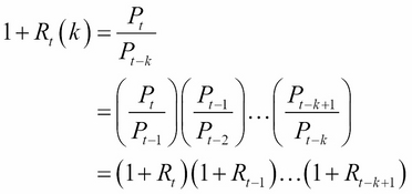
This is an example of a deterministic model, except that there is one caveat that we did not mention: you have to incorporate the inflation rate in the equation per year. If we include this in the preceding equation by assuming Ft is the inflation that corresponds to the return Rt, we will get the following equation:
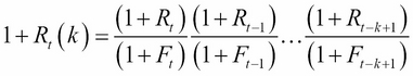
If we assume Ft = 0, then the previous equation would be applicable. Assume that we do not include inflation and ask this question: "with an initial investment of $10,000 in 2010 and a return rate of 6%, after how many years will my investment double?"
Let's try to find the answer with the Python program. In this program, we also have to add a straight line that is almost similar to y = 2x and see where it intersects the curve of the return values plotted on the y axis with the year running on the x axis. First, we will plot without the line to determine whether the invested value is almost doubled in 12 years. Then, we will calculate the slope of the line m = 10,000/12 = 833.33. Therefore, we included this slope value of 833.33 in the program to display both the return values and the straight line. The following code compares the return value overlap with the straight line:
import matplotlib.pyplot as plt

principle_value=10000  #invested amount
grossReturn = 1.06     # Rt

return_amt = []
x = []
y = [10000]
year=2010
return_amt.append(principle_value)
x.append(year)

for i in range(1,15):
  return_amt.append(return_amt[i-1] * grossReturn)
  print "Year-",i," Returned:",return_amt[i]

  year += 1
  x.append(year)
  y.append(833.33*(year-2010)+principle_value)

# set the grid to appear
plt.grid()

# plot the return values curve
plt.plot(x,return_amt, color='r')
plt.plot(x,y, color='b')

Year- 1 Returned: 10600.0
Year- 2 Returned: 11236.0
Year- 3 Returned: 11910.16
Year- 4 Returned: 12624.7696
Year- 5 Returned: 13382.255776
Year- 6 Returned: 14185.1911226
Year- 7 Returned: 15036.3025899
Year- 8 Returned: 15938.4807453
Year- 9 Returned: 16894.78959
Year- 10 Returned: 17908.4769654
Year- 11 Returned: 18982.9855834
Year- 12 Returned: 20121.9647184
Year- 13 Returned: 21329.2826015
Year- 14 Returned: 22609.0395575
After looking at the plot, you would wonder whether there is a way to find out how much money the banks that provide mortgage loans make. We'll leave this to you.

An interesting fact is that the curve intersects the line before 2022. At this point, the return value is exactly $20,000. However, in 2022, the return value will be approximately $20,121. Having looked at the gross returns, is it similar in stocks? Many stocks, especially of mature companies, pay dividends that must be accounted for in the equation.
If a dividend (or interest) Dt is paid prior to time t, then the gross return at time t is defined as follows:

Another example is a mortgage loan, where a certain amount of loan is borrowed from a financial institution at an interest rate. Here, for the purposes of understanding the nature of the business, we will select a loan amount of $350,000 at an interest rate of 5 percent on a 30-year term. This is a typical example of American Mortgage Loan (the loan amount and interest rate varies depending on the credit history and the market rate of interest of a loan seeker).
A simple interest calculation is known to be P (1 + rt), where P is the principal amount, r is the interest rate, and t is the term, so the total amount accrued at the end of 30 years is:

It turns out that by the end of 30 years, you would have paid more than twice the loan amount (we have not taken the real estate taxes into account in this calculation):
from decimal import Decimal
import matplotlib.pyplot as plt

colors = [(31, 119, 180),(174, 199, 232),(255,128,0),(255, 15, 14),
      (44, 160, 44),(152, 223, 138),(214, 39, 40),(255,173, 61),
      (148, 103, 189),(197, 176, 213),(140, 86, 75),(196, 156, 148),
      (227, 119, 194),(247, 182, 210),(127, 127, 127),
      (199, 199, 199),(188, 189, 34), (219, 219, 141),
      (23, 190, 207), (158, 218, 229)]

# Scale the RGB values to the [0, 1] range, which is the format matplotlib accepts.
for i in range(len(colors)):
    r, g, b = colors[i]
    colors[i] = (r / 255., g / 255., b / 255.)

def printHeaders(term, extra):
    # Print headers
    print "
Extra-Payment: $"+str(extra)+" Term:"+str(term)+" years"
    print "---------------------------------------------------------"
    print 'Pmt no'.rjust(6), ' ', 'Beg. bal.'.ljust(13), ' ',
    print 'Payment'.ljust(9), ' ', 'Principal'.ljust(9), ' ',
    print 'Interest'.ljust(9), ' ', 'End. bal.'.ljust(13)
    print ''.rjust(6, '-'), ' ', ''.ljust(13, '-'), ' ',
    print ''.rjust(9, '-'), ' ', ''.ljust(9, '-'), ' ',
    print ''.rjust(9, '-'), ' ', ''.ljust(13, '-'), ' '

def amortization_table(principal, rate, term, extrapayment, printData=False):
    xarr=[]
    begarr = []

    original_loan = principal
    money_saved=0
    total_payment=0
    payment = pmt(principal, rate, term)
    begBal = principal

    # Print data
    num=1
    endBal=1
    if printData == True: printHeaders(term, extrapayment)
    while  (num < term + 1) and (endBal >0):

        interest = round(begBal * (rate / (12 * 100.0)), 2)
        applied = extrapayment+round(payment - interest, 2)
        endBal = round(begBal - applied, 2)
        if (num-1)%12 == 0 or (endBal < applied+extrapayment):
          begarr.append(begBal)
          xarr.append(num/12)
          if printData == True:
              print '{0:3d}'.format(num).center(6), ' ',
              print '{0:,.2f}'.format(begBal).rjust(13), ' ',
              print '{0:,.2f}'.format(payment).rjust(9), ' ',
              print '{0:,.2f}'.format(applied).rjust(9), ' ',
              print '{0:,.2f}'.format(interest).rjust(9), ' ',
              print '{0:,.2f}'.format(endBal).rjust(13)
        total_payment += applied+extrapayment
        num +=1
        begBal = endBal
    if extrapayment > 0 :
      money_saved = abs(original_loan - total_payment)
      print '
Total Payment:','{0:,.2f}'.format(total_payment).rjust(13)
      print '  Money Saved:','{0:,.2f}'.format(money_saved).rjust(13)
    return xarr, begarr, '{0:,.2f}'.format(money_saved)

def pmt(principal, rate, term):
    ratePerTwelve = rate / (12 * 100.0)

    result = principal * (ratePerTwelve / (1 - (1 + ratePerTwelve) ** (-term)))

    # Convert to decimal and round off to two decimal
    # places.
    result = Decimal(result)
    result = round(result, 2)
    return result

plt.figure(figsize=(18, 14))

#amortization_table(150000, 4, 180, 500)
i=0
markers = ['o','s','D','^','v','*','p','s','D','o','s','D','^','v','*','p','s','D']
markersize=[8,8,8,12,8,8,8,12,8,8,8,8,8,8,8,8,8,8,8,8,8,8,8,8,8]

for extra in range(100,1700,100):
  xv, bv, saved = amortization_table(450000, 5, 360, extra, False)
  if extra == 0:
    plt.plot(xv, bv, color=colors[i], lw=2.2, label='Principal only', marker=markers[i], markersize=markersize[i])
  else:
    plt.plot(xv, bv, color=colors[i], lw=2.2, label="Principal plus$"+str(extra)+str("/month, Saved:$")+saved, marker=markers[i], markersize=markersize[i])
  i +=1


plt.grid(True)
plt.xlabel('Years', fontsize=18)
plt.ylabel('Mortgage Balance', fontsize=18)
plt.title("Mortgage Loan For $350,000 With Additional Payment Chart", fontsize=20)
plt.legend()
plt.show()
When this program is run, you would get the amortized schedule for every 12 months for all the cases of extra payment, starting from $100 to $1600. Here is just one of those cases:
Extra-Payment: $800 Term: 30 years
-----------------------------------------------------------------Pmt no   Beg. bal.   Payment   Principal   Interest    End. bal.     ------   ---------   -------   ---------   ---------   ------
  1      350,000.00  1,878.88* 1,220.55  1,458.33   348,779.45
 13      335,013.07  1,878.88  1,282.99  1,395.89   333,730.08
 25      319,259.40  1,878.88  1,348.63  1,330.25   317,910.77
 37      302,699.75  1,878.88  1,417.63  1,261.25   301,282.12
 49      285,292.85  1,878.88  1,490.16  1,188.72   283,802.69
 61      266,995.41  1,878.88  1,566.40  1,112.48   265,429.01
 73      247,761.81  1,878.88  1,646.54  1,032.34   246,115.27
 85      227,544.19  1,878.88  1,730.78    948.10   225,813.41
 97      206,292.20  1,878.88  1,819.33    859.55   204,472.87
109      183,952.92  1,878.88  1,912.41    766.47   182,040.51
121      160,470.74  1,878.88  2,010.25    668.63   158,460.49
133      135,787.15  1,878.88  2,113.10    565.78   133,674.05
145      109,840.70  1,878.88  2,221.21    457.67   107,619.49
157       82,566.78  1,878.88  2,334.85    344.03    80,231.93
169       53,897.49  1,878.88  2,454.31    224.57    51,443.18
181       23,761.41  1,878.88  2,579.87     99.01    21,181.54
188        5,474.98  1,878.88  2,656.07     22.81     2,818.91
189        2,818.91  1,878.88  2,667.13     11.75       151.78

* $1878.88 includes $1078.88 plus $800 extra payment towards principal
Total Payment: $504,526.47 Money Saved: $154,526.47
Approximately after 15 years 10 months, one can pay off in half the time.
The Python code results in the following plot that compares the additional savings with principal savings on a mortgage payment:

The preceding plot shows the mortgage balance dropping earlier than the 30 years by paying an additional amount against the principal amount.
The monthly payment for a fixed rate mortgage is the amount paid by the borrower every month to ensure that the loan is paid in full with interest at the end of its term. The monthly payment depends on the interest rate (r) as a fraction, the number of monthly payments (N), which is called the loan's term, and the amount borrowed (P), which is called the loan's principal; when you rearrange the formula for the present value of an ordinary annuity, we get the formula for the monthly payment. However, every month, if an extra amount is paid along with the fixed monthly payment, then the loan amount can be paid off in a much shorter time.
In the following chart, we have attempted to use the money saved from the program and plot that money against the additional amount in the range of $500 to $1300. If we see carefully, with an additional amount of $800, you can save almost half the loan amount and pay off the loan in half the term.

The preceding plot shows the savings for three different loan amounts, where the additional contribution is shown along the x axis and savings in thousands is shown along the y axis. The following code uses a bubble chart that also visually shows savings toward additional amount toward the principal on a mortgage loan:
import matplotlib.pyplot as plt

# set the savings value from previous example
yvals1 = [101000,111000,121000,131000,138000, 143000,148000,153000,158000]
yvals2 = [130000,142000,155000,160000,170000, 180000,190000,194000,200000]
yvals3 = [125000,139000,157000,171000,183000, 194000,205000,212000,220000]
xvals = ['500','600','700', '800', '900','1000','1100','1200','1300']

#initialize bubbles that will be scaled
bubble1 = []
bubble2 = []
bubble3 = []

# scale it on something that can be displayed
# It should be scaled to 1000, but display will be too big
# so we choose to scale by 5% (divide these by 20 again to relate
# to real values)

for i in range(0,9):
  bubble1.append(yvals1[i]/20)
  bubble2.append(yvals2[i]/20)
  bubble3.append(yvals3[i]/20)

#plot yvalues with scaled by bubble sizes
#If bubbles are not scaled, they don't fit well
fig, ax = plt.subplots(figsize=(10,12))
plt1 = ax.scatter(xvals,yvals1, c='#d82730', s=bubble1, alpha=0.5)
plt2 = ax.scatter(xvals,yvals2, c='#2077b4', s=bubble2, alpha=0.5)
plt3 = ax.scatter(xvals,yvals3, c='#ff8010', s=bubble3, alpha=0.5)

#Set the labels and title
ax.set_xlabel('Extra Dollar Amount', fontsize=16)
ax.set_ylabel('Savings', fontsize=16)
ax.set_title('Mortgage Savings (Paying Extra Every Month)',
        fontsize=20)

#set x and y limits
ax.set_xlim(400,1450)
ax.set_ylim(90000,230000)

ax.grid(True)
ax.legend((plt1, plt2, plt3), ('$250,000 Loan', '$350,000 Loan',
     '$450,000 Loan'), scatterpoints=1, loc='upper left',
      markerscale=0.17, fontsize=10, ncol=1)

fig.tight_layout()
plt.show()
By creating a scatter plot, it is much easier to view which loan category would offer more savings compared to others, but to keep it simple, we will compare only three loan amounts: $250,000, $350,000, and $450,000.
The following plot is the result of a scatter plot that demonstrates the savings by paying extra every month:
