
The clustering coefficient of a node or a vertex in a graph depends on how close the neighbors are so that they form a clique (or a small complete graph), as shown in the following diagram:

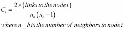
There is a well known formula to cluster coefficients, which looks pretty heavy with mathematical symbols. However, to put it in simple words, take a look at the following equation:

This involves keeping track of the links at every vertex and calculating the clustering index at every vertex, where the neighbor of a node in the most obvious sense is a node that is only one link away from that node. Clustering index calculation is shown here:

The following code illustrates how you can show the characters of the Les Miserables novel and how each character is associated or connected to other characters:
import networkx as nx
from pylab import rcParams
rcParams['figure.figsize'] = 12, 12

G = nx.read_gml('/Users/kvenkatr/Downloads/lesmiserables.gml', relabel=True)
G8= G.copy()

dn = nx.degree(G8)

for n in G8.nodes():
  if dn[n] <= 8:
    G8.remove_node(n)

pos= nx.spring_layout(G8)
nx.draw(G8, node_size=10, edge_color='b', alpha=0.45, font_size=9, pos=pos)
labels = nx.draw_networkx_labels(G8, pos=pos)

def valuegetter(*values):
    if len(values) == 1:
        item = values[0]
        def g(obj):
            return obj[item]
    else:
        def g(obj):
            return tuple(obj[item] for item in values)
    return g

def clustering_coefficient(G,vertex):
    neighbors = G[vertex].keys()
    if len(neighbors) == 1: return -1.0
    links = 0
    for node in neighbors:
        for u in neighbors:
            if u in G[node]: links += 1
    ccoeff=2.0*links/(len(neighbors)*(len(neighbors)-1))
    return links, len(neighbors),ccoeff

def calculate_centrality(G):
    degc = nx.degree_centrality(G)
    nx.set_node_attributes(G,'degree_cent', degc)
    degc_sorted = sorted(degc.items(), key=valuegetter(1), reverse=True)
    for key, value in degc_sorted[0:10]:
        print "Degree Centrality:", key, value
    return G, degc

print "Valjean", clustering_coefficient(G8,"Valjean")
print "Marius", clustering_coefficient(G8,"Marius")
print "Gavroche", clustering_coefficient(G8,"Gavroche")
print "Babet", clustering_coefficient(G8,"Babet")
print "Eponine", clustering_coefficient(G8,"Eponine")
print "Courfeyrac", clustering_coefficient(G8,"Courfeyrac")
print "Comeferre", clustering_coefficient(G8,"Combeferre")
calculate_centrality(G8)
There are two results of the preceding code; the first part is the textual output that gets printed, whereas the second part is the network diagram that gets plotted, as shown in the following code and diagram:
#Text Results printed
Valjean (82, 14, 0.9010989010989011)
Marius (94, 14, 1.032967032967033)
Gavroche (142, 17, 1.0441176470588236)
Babet (60, 9, 1.6666666666666667)
Eponine (36, 9, 1.0)
Courfeyrac (106, 12, 1.606060606060606)
Comeferre (102, 11, 1.8545454545454545)

Degree Centrality: Gavroche 0.708333333333
Degree Centrality: Valjean 0.583333333333
Degree Centrality: Enjolras 0.583333333333
Degree Centrality: Marius 0.583333333333
Degree Centrality: Courfeyrac 0.5
Degree Centrality: Bossuet 0.5
Degree Centrality: Thenardier 0.5
Degree Centrality: Joly 0.458333333333
Degree Centrality: Javert 0.458333333333
Degree Centrality: Feuilly 0.458333333333
The graph results are shown here below.

Clearly among all, so far we have found that Comeferre happens to have a larger clustering coefficient (0.927). Often, when we plot a large graph in two dimensions, it is not easy to visually see the clustering coefficient.