
6
Error Control Coding
Thomas E. Fuja
The Fundamentals of Binary Block Codes
Coding Gain, Hard Decisions, and Soft Decisions
The Fundamentals of Convolutional Codes
6.5 Low-Density Parity Check Codes
6.6 Coding and Bandwidth-Efficient Modulation
Bit-Interleaved Coded Modulation
6.1 Introduction
Error control coding is a branch of communication engineering that addresses the problem of how to make digital transmission more reliable—how to recover uncorrupted data at the receiver even in the presence of significant corruption of the transmitted signal.
The modern genesis of error control coding has its roots in the post–World War II work of Claude Shannon (who proved the existence of “good codes” but did not indicate how to find them [1]) and Marcel Golay and Richard Hamming (who published the first explicit descriptions of “error correcting codes” based on parity checks [2,3]).
Error control codes make digital transmission more reliable by the careful introduction of redundancy into the transmitted signal. The simplest example of such a scheme might be one in which every data bit to be conveyed to the receiver is transmitted three times—that is, a logical “1” would be transmitted as “111” and a logical “0” as “000.” The redundancy introduced by repeating each bit can be exploited at the receiver to make errors in the estimated data less likely—by, for instance, making a decision on each of the three bits individually and then taking a “vote” of the three decisions to arrive at an estimate of the associated data bit. In such a scheme, as long as not more than one bit is corrupted out of every three-bit “codeword,” the receiver will correctly decode the data; thus, this is a (very simple) one-error correcting code.
Error control schemes can be broadly classified into two categories:
Forward error control (FEC) codes, in which sufficient redundancy is incorporated into the “forward” (transmitter-to-receiver) transmission to enable the receiver to recover the data well enough to meet the requirements of the application.
Automatic repeat request (ARQ), in which enough redundancy is incorporated into the forward transmission to enable the receiver to detect the presence of corruption—but not enough to reliably estimate the data from the (corrupted) received signal. ARQ schemes employ a retransmission strategy in which the receiver alerts the transmitter (via an “ACK/NACK” protocol on a feedback channel) of the need to retransmit the corrupted data.

FIGURE 6.1 The communication theorist's “coat of arms,” wherein the error control (or “channel”) encoder introduces redundancy that is then exploited by the channel decoder to enhance data integrity in the presence of channel noise.
A classic depiction of a digital communication system employing FEC is shown in Figure 6.1. Data generated by the source is first compressed by a source encoder—tasked with removing redundancy to produce an efficient binary representation of the data—and then passed through the error control (or “channel”) encoder, which adds redundancy to enable robust recovery by the error control (or “channel”) decoder at the receiver. These seemingly conflicting operations—removing redundancy only to then add redundancy—are required because the “natural” redundancy that occurs in (for instance) speech or video signals is not sufficiently structured that it can be exploited at the receiver as effectively as the well-structured redundancy introduced by the error control encoder.
Figure 6.1 suggests that error control is carried out solely at the physical layer, which is not the case. Most notably, when ARQ is employed, the retransmission function is part of the processing at the (data) link layer.
The rest of this chapter discusses a multitude of error control techniques that have been implemented in mobile communication systems. While there are many different approaches, all error control schemes have this in common: They add structure to the transmitted signal in a way that limits what can be transmitted, compared with uncoded transmission. In a coded system, there are only certain signals that are valid and can thus be transmitted; since the receiver knows what those valid signals are, it can use that knowledge to select the valid sequence that is “most like” what it observes. From another perspective, coding exaggerates the differences between distinct data sequences in their transmitted form, making it easier to discern one from the other at the receiver.
6.2 Block Codes
Classic error control codes can be split into block codes and convolutional codes. In this section, we explain block codes.
6.2.1 The Fundamentals of Binary Block Codes
The very simple code described in the introduction—in which “1” is transmitted as “111” and “0” as “000”—is called a block code. It is given this name because a block of data—in this case, one bit—is represented with another (longer) block of transmitted bits—in this case, three bits. The two valid 3-bit sequences—“000” and “111”—are called the codewords of this code, and its blocklength is n = 3. We refer to this as a rate-1/3 code because there is one data bit for every three encoded (or transmitted) bits.
Generalizing, an (n, k) binary block code is one in which k data bits are represented with an n-bit codeword; thus, there are 2k different codewords, each n bits long, where n > k. The rate of the resulting code is R = k/n data bits per encoded bit.
As noted above, error control codes make it easier to differentiate between different “valid” transmitted signals. With regard to block codes, this property is captured (to first order) by the code's minimum distance, which is defined as the fewest number of coordinates in which two codewords differ. (So the trivial code in the introduction is a (3,1) code with a minimum distance of dmin = 3, because every pair of codewords—and there are only two codewords—differ in at least three coordinates.) The Hamming distance between any two n-tuples is defined as the number of coordinates in which they differ, and the Hamming weight of a particular vector is the number of its nonzero components.
As a slightly less simple example, consider the (n = 7, k = 4) Hamming code below.
0000 → 0000000 |
0100 → 0100101 |
1000 → 1000110 |
1100 → 1100011 |
0001 → 0001111 |
0101 → 0101010 |
1001 → 1001001 |
1101 → 1101100 |
0010 → 0010011 |
0110 → 0110110 |
1010 → 1010101 |
1110 → 1110000 |
0011 → 0011100 |
0111 → 0111001 |
1011 → 1011010 |
1111 → 1111111 |
Here, “0010 → 0010011” (for instance) means that the data 4-tuple “0010” is represented with the 7-bit codeword “0010011.” There are 24 = 16 codewords, each of length n = 7, and the rate of this code is R = 4/7 data bits per encoded bit. Moreover, careful inspection reveals that every pair of codeword differs in at least dmin = 3 places, so this is a code with a minimum distance of three.
The significance of a block code's minimum distance is most clear if we think in terms of the decoder. Suppose that a codeword is transmitted and that each bit has independent probability p of being “flipped”—that is, of being sufficiently corrupted that a transmitted “1” is misinterpreted by the receiver as a “0” or vice versa. Then, assuming that p < 1/2, most bits should be received correctly, and so the most likely transmitted codeword is the one that disagrees with the received signal in the fewest coordinates—that is, the “closest” codeword in terms of Hamming distance. A decoder that estimates data based on this principle is called a minimum distance—or maximum-likelihood (ML)—decoder. ML decoding is optimal, assuming that the data are a sequence of independent, identically distributed bits, each equally likely to be a “1” or a “0.”
As an example, suppose that the codeword c = [1011010] is transmitted but y = [1010010] is received, with a single error in the fourth coordinate. If you compare y to every codeword, you find that the codeword closest to y is, in fact, c = [1011010]; thus, the ML decoder's estimate of the transmitted codeword (and the associated data) is, in fact, correct. In contrast, if c = [1011010] is transmitted but y′ = [1011001] is received—the last two bits are “flipped”—then the closest codeword to y′ is c′ = [1001001], which means that the ML decoder will assume that c′ was transmitted and will estimate the associated data to be (the incorrect) “1001” rather than (the correct) “1011”—that is, there will be a decoding error.
A t-error correcting binary block code is one for which minimum distance decoding will yield a correct estimate of the transmitted codeword provided no more than t errors have occurred; thus, a t-error correcting code must have the property that, if you “flip” any set of t or fewer bits in any codeword c, the resulting vector is still “closer” to c—that is, disagrees in fewer places—than to any other codeword. This leads to the relationship: A t-error correcting code must have a minimum distance dmin that satisfies
Equivalently, a code with minimum distance dmin can correct up to t = ⌊(dmin − 1)/2⌋ errors, where “⌊·⌋” indicates the floor function.
A close examination of the 16 codewords in the above (7,4) Hamming code reveals at least two more properties worth noting:
If you add any two codewords together—here, “add” means component-wise XOR—then you get another codeword. In the language of mathematics, the code forms a linear vector space over the binary field {0,1}, and so we say this is a linear code. One consequence of linearity is that the code's minimum distance is equal to its minimum nonzero codeword weight.
The first k = 4 bits of every codeword are identical to the associated k data bits. In the language of coding, the encoder is systematic on the first k positions.
Linear codes are useful because their algebraic structure enables simpler decoding and simpler analysis. Moreover, there are matrices associated with a linear block code that facilitate the encoding and decoding procedures. The generator matrix for an (n, k) binary block code is a k × n matrix G with binary entries such that its rows form a basis for the code—that is, the code is equal to the set of all sums (or “linear combinations”) of the rows of G. This is expressed mathematically as C = {c: c = xG for some x ∈ {0,1}k}. A generator for the above (7,4) code is given by
Similarly, a parity check matrix for an (n,k) binary code is an (n – k) × n binary matrix whose rows form a basis for the null space of the code—that is, H is a parity check matrix for a code C if and only if C = {c: c ∈ {0,1}n, cHT = 0}, where 0 is the (n – k)-tuple with all zero entries. The parity check matrix for the (7,4) code above is given by
Note that the rows of the parity check matrix describe the parity constraints that must be satisfied by every codeword. For example, the first row of H above indicates that the first, second, fourth, and fifth bits in every codeword must have even parity—that is, must contain an even number of 1’s; the other two rows of H indicate two other parity constraints that must be satisfied by every codeword. More generally, the (n – k) rows of a parity check matrix describe (n − k) parity constraints that characterize the code.
The generator and parity check matrices are used in the encoding and decoding operations, respectively. With regard to encoding, the data vector x ∈ {0,1}k is mapped onto the associated codeword c = xG. With regard to decoding, let y ∈ {0,1}n denote a (possibly corrupted) received binary n-tuple—that is, assume that codeword c was transmitted but y = x + e was received, where e ∈ {0,1}n is the a noise vector. Then, a typical “first step” in the decoding process is to compute the syndrome s associated with the received vector:
The syndrome s is computed from the received vector y but depends only on the error e—not on the transmitted codeword. The syndrome for a binary code is a binary (n – k)-tuple—that is, s ∈ {0,1}n−k—and in syndrome decoding the syndrome s is first computed, and from s an estimate of the error vector e is formed. (Of course, once the error vector is estimated it is trivial to estimate the transmitted codeword by subtracting the error estimate from the received vector.)
There is a one-to-one relationship between correctable error patterns and syndromes; for every syndrome s, there are many possible choices of e satisfying s = eHT, but the decoder is capable of correcting exactly one of them. This observation—coupled with the observation that a t-error correcting code can correct (at least) every error pattern affecting t or fewer bits—leads to the following bound, called the Hamming bound:
Any binary (n,k) t-error correcting linear code must have parameters that satisfy the Hamming bound; codes that satisfy the Hamming bound with equality are called perfect codes. Similarly, the Singleton bound states that any (n,k) code with minimum distance dmin must have parameters that satisfy
Codes that satisfy the Singleton bound with equality are called maximum distance separable codes.
The advantage of syndrome decoding lies in how it reduces the dimensionality of the decoding problem. The job of the decoder is to find the codeword c that is closest to the received vector y; without using the code's structure, this could be done (in theory, if not in practice) with a table containing 2n entries: the received vector y is used as an index into the table, and the associated entry contains the codeword closest to y. However, if we first compute s = yHT we can now use s as an index into a table containing the 2n−k correctable error patterns. For a (63,57) Hamming code, this reduces the required table from one containing 263 = 9.22 × 10¹⁸ entries to one containing only 26 = 64 entries. Of course, for many practical codes this reduction in dimensionality still leaves a formidable problem: A (1023,923) 10-error correcting code produces a 100-bit syndrome, still far too large for a brute-force approach.
The (7,4) code used throughout this section is a Hamming code—one of a class of codes presented by Richard Hamming in 1950. More generally, a Hamming code is an (n = 2r − 1, k = 2r − 1 − r) binary linear block code for any choice of r = 2,3,4, … . Hamming codes are single-error correcting codes with minimum distance dmin = 3. The Hamming code with blocklength n = 2r − 1 is constructed using a parity check matrix with columns that are the 2r − 1 distinct non-all-zero binary r-tuples.
It is possible to extend a Hamming code by adding one additional redundant bit to every codeword to guarantee that every codeword has even parity—that is, an even number of ones. This converts the (2r − 1, 2r − 1 − r) code into a (2r, 2r − 1 − r) extended code—for example, the (7,4) Hamming code becomes the (8,4) extended Hamming code. Extending the code in this way increases the minimum distance of the code from dfree = 3 to dfree = 4. This additional minimum distance can be exploited to add a new capability—to not only correct any single error but also simultaneously detect (without miscorrecting) any double error. More generally, a block code is capable of correcting t errors and simultaneously detecting e ≥ t errors provided its minimum distance satisfies dmin ≥ t + e + 1.
6.2.2 Reed–Solomon Codes
The single-error correcting Hamming codes used to illustrate coding basics in the last section were the first practical “error correcting codes.” The development of a general technique for constructing t-error correcting codes for t > 1 took another decade—until the unveiling of BCH codes [4,5] and Reed–Solomon codes [6] in 1959 and 1960. Reed–Solomon codes continue to be used today in a wide array of wireless (and other) applications, so we briefly describe their structure.
A Reed–Solomon code is a nonbinary code, meaning that each codeword from a Reed–Solomon code with blocklength n consists of n nonbinary symbols. An (n,k) Reed–Solomon code with minimum distance dmin protects k data symbols by adding n − k redundant symbols such that every pair of codewords differs in at least dmin symbols. Moreover, the symbols are drawn from a nonbinary field, briefly explained below.
A “field” is a set with two operations—addition and multiplication—that satisfy the “usual” commutative, associative, and distributive properties and also contain additive and multiplicative identities as well as additive inverses and (for nonzero elements) multiplicative inverses. (The set of real numbers form a field under the usual notions of addition and multiplication, as do the set of complex numbers; the set of all integers do not because there are no multiplicative inverses.) A finite field (or Galois field) is a field with a finite number of elements; for instance, the binary field—containing just the elements {0,1}, with addition and multiplication performed modulo two—is a finite field.
Let GF(q) denote a field with q elements; then it is possible to construct the field GF(pm) for any prime number p and any positive integer m, and it is impossible to construct a field with q elements if q is not a power of a prime. To construct the field GF(p) for prime p, the field consists of the integers {0,1,2, …, p − 1} and both addition and multiplication are performed modulo p. To construct the field GF(pm) for m > 1 requires more subtlety; the field elements of GF(pm) are the polynomials of degree at most m − 1, with coefficients drawn from GF(p). There are pm such polynomials, and if addition and multiplication are defined appropriately, then the resulting structure is a field. Here, “appropriately” means that addition is performed in the “usual” polynomial fashion, component-wise modulo p, while multiplication is performed in polynomial fashion, but the result is reduced modulo π(x), where π(x) is an irreducible polynomial with coefficients in GF(p) of degree exactly m. An irreducible polynomial is one that cannot be factored; it is analogous among polynomials to a prime number among integers.
For details on the construction of finite fields, the reader is referred to any textbook on error control coding or modern algebra. What is important to understand now is that each field element of GF(pm) can be represented as a symbol made up of m digits drawn from {0,1,2,…, p − 1}—that is, the m coefficients of the field element polynomial.
In practice, Reed–Solomon codes are designed over GF(2m), so each symbol in a Reed–Solomon codeword can take one of 2m values and is represented as an m-bit symbol. Of particular interest are Reed–Solomon codes over GF(256), because 256 = 28 and therefore each codeword from an (n,k) Reed–Solomon code over GF(256) is n bytes long—with k data bytes and n – k redundant bytes and each byte consisting of eight bits. Such a code has 256k codewords, and the rate is R = k/n data bytes per encoded byte.
An (n,k) Reed–Solomon code over GF(q) has blocklength n = q − 1 and minimum distance dmin = n – k + 1. (So Reed–Solomon codes are maximum distance separable codes as defined in Section 6.3.) Such a code is specified by its parity check matrix:
Here, α is a primitive element of the field GF(q). That means that all of the nonzero elements of GF(q) can be written as powers of α—that is, GF(q) = {0, α0 = 1, α1, α2, α3, …, αq−2}. As with binary linear codes, the parity check matrix for an (n,k) Reed–Solomon code is an (n – k) × n array, so in H above, we have r = n – k.
The integer j in the above description of H is often (but not always) set to j = 1. If we think of the components of a codeword c = [c0, c1, c2, …, cn−1] as representing the coefficients of a polynomial c(x) = c0 + c1x + c2x2 + … + cn−1xn−1, then the relationship cHT = 0 is equivalent to the relationship c(αj) = c(αj+1) = c(αj+2) = … = c(αj+r−1) = 0. This suggests an equivalent definition for Reed–Solomon codes: For a fixed integer j and a fixed redundancy r = n – k, an (n = q − 1, k = n – r) Reed–Solomon code over GF(q) consists of all polynomials over GF(q) of degree n − 1 or less that have r consecutive powers of a primitive element α as roots: αj, αj+1, αj+2, …, αj+r−1. Such a code has a minimum distance dmin = r + 1 and so is capable of correcting all error patterns affecting not more than ⌊ r/2⌋ symbols.
A few observations complete our discussion on Reed–Solomon codes:
While, strictly speaking, a Reed–Solomon code over GF(q) has a blocklength n = q − 1, it is possible to shorten a Reed–Solomon code—or any other code, for that matter—by arbitrarily setting some (say s) of the k information symbols to zero and then simply not transmitting them; as a result, an (n,k) code with minimum distance dmin is transformed into an (n – s, k – s) code with minimum distance at most dmin. (For Reed–Solomon codes, the minimum distance of the shortened code is unchanged.) For example, the advanced television systems committee (ATSC) standard for terrestrial digital television broadcast employs a (207,187) shortened Reed–Solomon code over GF(256). It is obtained by shortening the (255,235) Reed–Solomon code; the resulting code adds r = 20 bytes of redundancy to k = 187 bytes of data in a way that guarantees the correction of up to t = 10 byte errors in any codeword.
Because Reed–Solomon codes are organized on a symbol (rather than bit) basis, they are well suited to correcting bursty errors—that is, errors highly correlated in time. To illustrate: A burst of (say) 15 corrupted bits can affect no more than three 8-bit symbols and so can be corrected with a relatively modest 3-error correcting Reed–Solomon code over GF(256). This effectiveness with regard to bursty noise can be enhanced through the use of interleaving—that is, by interspersing the symbols from different codewords among each other, thereby spreading out the effect of the error burst over multiple codewords. (Example: If a code over GF(256) is interleaved to depth three, then that same 15-bit error burst would affect at most one symbol in each of three different codewords, and therefore it would be ameliorated by an even simpler 1-error correcting code.)
6.2.3 Coding Gain, Hard Decisions, and Soft Decisions
The benefits of channel coding are typically expressed in terms of a coding gain—an indication of how much the transmitted power can be reduced in a coded system without a loss in performance, relative to an uncoded system. Coding gain depends not only on the code that is used but also on whether hard-decision decoding or soft-decision decoding is employed.
In hard-decision decoding, the demodulator makes a “hard decision” about each transmitted bit; those decisions are then conveyed to the FEC decoder which corrects any errors made by the demodulator. In soft-decision decoding, the FEC decoder is provided not with hard decisions it must accept or correct, but rather with “soft” information that reflects the “confidence” with which the demodulator would make such a decision.
As an example, consider binary phase shift keying (BPSK) modulation in the presence of additive white Gaussian noise (AWGN). For each transmitted bit, the receiver observes a matched filter output Y of the form , where the sign of indicates whether the transmitted bit is a “0” or “1,” E is the energy of the transmitted pulse, and Z is a 0-mean Gaussian random variable with variance N0/2. In a hard-decision system, the demodulator estimates the transmitted bit based on whether Y is positive or negative, and it then passes that estimate to the decoder. When soft-decision decoding is employed, the FEC decoder gets direct access to the “soft information” contained in the unquantized (or very finely quantized) Y. More generally, in soft-decision decoding, the channel decoder is given access to the demodulator's matched filter outputs—typically quantized to several bits of precision.
To compare coded and uncoded transmission, the signal-to-noise ratio is typically expressed as Eb/N0, where Eb is the average energy per data bit. If the (average) energy of each transmitted pulse is E, and each pulse conveys (on average) R data bits, then Eb = E/R. Displaying performance as a function of Eb/N0 facilitates a fair(er) comparison because it includes the energy penalty that FEC codes pay to transmit their redundancy. However, these comparisons are not wholly fair because they do not address the bandwidth penalty that FEC can incur for a fixed modulation scheme; for instance, in transmitting data over a BPSK-modulated channel, using a (7,4) Hamming code requires 75% more bandwidth than uncoded transmission, because the transmitted bits (including redundancy) must be sent 75% faster after encoding if the data are to be delivered just as fast as in the uncoded case. The question of how to design codes without bandwidth expansion is addressed in Section 6.6.

FIGURE 6.2 The bit error rate of a (7,4) Hamming code—with hard-decision and soft-decision decoding—compared with uncoded transmission for a BPSK-modulated AWGN channel.
Figure 6.2 shows the performance of the simple (7,4) Hamming code assuming BPSK modulation and an AWGN channel. It includes the performance with both hard-decision and soft-decision decoding, and uncoded transmission is included for comparison. Observe that hard-decision decoding of the Hamming code provides approximately 0.45 dB of coding gain over uncoded transmission at a bit error rate of 10−5, while soft-decision decoding offers an additional 1.4 dB of gain. These coding gains mean that coded transmission requires only 90% (resp., 65%) of the transmitted power required for uncoded transmission to obtain a bit error rate (BER) of 10−5 when hard-decision (resp., soft-decision) decoding is used.
As a rule of thumb, at high signal-to-noise ratio (SNR), there is approximately a 2 dB gain associated with soft-decision decoding, compared to hard-decision decoding [7]. However, soft-decision decoding of algebraically constructed block codes is computationally complex; indeed, it was shown in Reference 8 that optimal (ML) soft-decision decoding of Reed–Solomon codes is NP-hard, although suboptimal algorithms that exploit soft information remain a subject of considerable research interest [9]. (ML soft-decision decoding selects as its estimate of the transmitted codeword the one that minimizes the Euclidean distance between the received signal and the modulated codeword.)
The formidable challenge of exploiting soft information in the decoding of block codes is one reason why other FEC techniques have evolved—techniques that are more accommodating to soft-decision decoding. One of the most fundamental of those other techniques is convolutional coding.
6.3 Convolutional Codes
Convolutional codes first appeared in a 1955 paper by Peter Elias [10]. Their popularity in practical digital communication systems came about largely because of the discovery in 1968 of a well-suited soft-decision decoding algorithm—the Viterbi algorithm.
6.3.1 The Fundamentals of Convolutional Codes
While an (n,k) binary block code assigns a discrete n-bit codeword to every discrete k-bit data block, an (n,k) binary convolutional code is one in which a “sliding block encoder” is used to generate n encoded sequences based on k data sequences. As a simple, illustrative example, consider the convolutional encoder in Figure 6.3. Here, the binary data sequence {x1, x2, x3, …} is used to generate the encoded sequences and according to these rules:
(As before, “ + ” indicates the binary XOR operation.) Thus, this is a (2,1) convolutional encoder because it accepts k = 1 binary sequence as an input and produces n = 2 binary-encoded sequences. More generally, an (n,k) convolutional encoder is a k-input, n-output, time-invariant, linear, causal, finite-state binary sequential circuit.
Just as linear block codes have generator and parity check matrices, so do convolutional codes. These representations employ the D-transform of a binary sequence: The D-transform of the binary sequence {b0, b1, b2, …} is given by B(D) = b0 + b1D + b2D2 + …. Then, a convolutional encoder takes k data sequences—represented by x = [x1(D), x2(D), …, xk(D)], where xi(D) is the D-transform of the ith data sequence—and produces n encoded sequences, represented by y = [y1(D), y2(D), …, yn(D)]; the generator matrix G for such an encoder is a k × n matrix with entries that are rational functions in D such that y = xG. For example, the generator of the convolutional encoder shown in Figure 6.3 is given by G = [1 + D2 1 + D + D2].
Convolutional encoders are finite-state machines. At any point in time, a convolutional encoder is in a particular “state” determined by its memory values; the encoder then accepts k input bits (one from each of the k data sequences) and produces an n-bit output while transitioning to a new state. This behavior is captured by a state diagram; the state diagram associated with the encoder in Figure 6.3 is shown in Figure 6.4a. The state of this particular encoder is determined by the previous two input bits—that is, when the encoder accepts input bit xi, it is in the state determined by xi−1 and xi−2, because there are ν = 2 memory elements in the encoder; thus, this is a 4-state encoder. In general, a convolutional encoder with ν bits of memory has 2ν states, and ν is referred to as the code's constraint length, an indicator of the code's complexity. In Figure 6.4a, each of the four states is represented by a node in a directed graph; the branches between the nodes indicate the possible transitions, and the label “x/y(1) y(2)” denotes the input (x) that causes the transition along with the two-bit output (y(1) y(2)) that results.
An alternative representation of a convolutional encoder is the trellis diagram—a graph that includes the same state and transition information as the state diagram but also includes a time dimension. The trellis diagram for the (2,1) convolutional encoder under consideration is shown in Figure 6.4b; it shows, for instance, that when the encoder is in state 1 (corresponding to xi−1 = 1, xi−2 = 0) then an input of “0” (resp., “1”) will cause a transition to state 2 (resp., 3) and produce an output of “01” (resp., “10”).
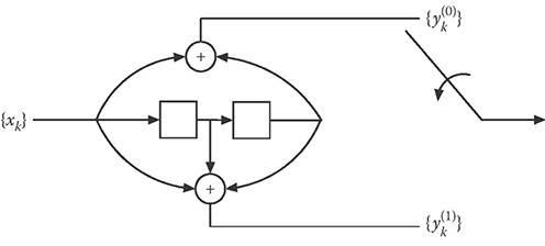
FIGURE 6.3 An encoder for a (2,1) convolutional code; the generator is G = [1 + D2 1 + D + D2].

FIGURE 6.4 (a) The state diagram and (b) trellis diagram of the convolutional encoder from Figure 6.2.
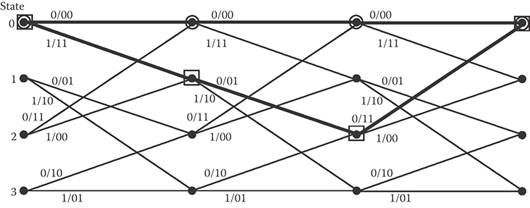
FIGURE 6.5 Two paths through the trellis illustrating that the free distance of the code is dfree = 5.
The free distance of a convolutional code is the minimum Hamming distance between any two valid encoded sequences; like the minimum distance of a block code, the free distance of a convolutional code indicates how “far apart” two distinct encoded sequences are guaranteed to be. Moreover, because of the assumed linearity of convolutional codes, the free distance of a code is equal to the minimum Hamming weight of any sequence that diverges from the all-zero sequence and then remerges. This is seen in Figure 6.5, where it is shown that the convolutional code with generator G = [1 + D2 1 + D + D2] has a minimum distance of dfree = 5.
6.3.2 The Viterbi Algorithm
In 1967, Dr. Andrew Viterbi published a paper [11] in which he presented an “asymptotically optimum decoding algorithm” for convolutional codes—an algorithm that transformed how digital communication systems were designed.
The Viterbi algorithm as applied to the decoding of convolutional codes is best understood as finding the “best path” through the code trellis. Referring to Figures 6.4b and 6.5, every branch in the trellis corresponds to the encoding of k data bits and the transmission of n channel bits; thus, there are 2kL paths of length L through the trellis—that is, 2kL paths made up of L branches—that start in a particular state at a particular point in time. Finding the “best path” through a brute force approach would quickly become unwieldy for even moderate values of L, since it would require comparing an observed signal of length L with 2kL candidate paths.
The key insight of the Viterbi algorithm is this: The relevant metrics—that is, the relevant measures of what constitutes the “best path”—are additive over the length of the received sequence, and so when two paths “merge” into the same state, only one path—the best one entering that state—can remain a candidate for the title of “best path.” So, instead of keeping track of 2kL candidate paths of length L, we need to retain only 2ν—one for each of the 2ν states, because only the best path entering each state is a “survivor.”
The ML metric is the log-likelihood function; if x is transmitted and y is received, then log[p(y|x)] reflects how likely y is to have been produced by x. Note that if the channel is “memoryless”—that is, each successive transmission is affected independently by the channel noise—then p(y|x) = Π p(yi|xi) and the metric log[p(y|x)] = Σ log[p(yi|xi)] is indeed additive. For additive Gaussian noise, maximizing this metric is equivalent to minimizing the cumulative squared Euclidean distance between x and y.
6.4 Turbo Codes
At the 1993 International Conference on Communications in Geneva, Switzerland, a groundbreaking new approach to error control coding was unveiled [12]. In a paper titled “Near Shannon Limit Error Correcting Coding and Decoding: Turbo Codes” by Berrou, Glavieux, and Thitimajshima, the authors demonstrated good performance—a bit error rate of 10−5—with a rate-1/2 code at an Eb/N0 value of only 0.7 dB on the BPSK-modulated AWGN channel. That is only 0.5 dB away from the Eb/N0 limit mandated by Shannon's capacity result for BPSK-modulated signaling.
The approach taken in Reference 12 (and in the follow-up journal paper [13]) was to use parallel concatenated convolutional encoders with an iterative decoder structure—an approach widely referred to as turbo (de-)coding.
The now-classic structure of a turbo encoder is shown in Figure 6.6. Two encoders—both recursive systematic convolutional encoders—are placed in parallel. The same input data are applied to both encoders—to the first encoder in unaltered form and to the second encoder after it has passed through an interleaver π. The “job” of the interleaver is to change the order in which the bits are encoded in a pseudo-random—that is, random-looking but deterministic—fashion.
The encoder unveiled in the 1993 paper is shown in Figure 6.7; it uses two rate-1/2 convolutional encoders, each with generator G = [1(1 + D4)/(1 + D + D2 + D3 + D4)]. The encoder thus produces three bitstreams—one consisting of the systematic data bits and two parity streams, one formed by the original data, and the other formed by the interleaved data. As such, this is a rate-1/3 code; however, in References 11 and 12, half of the parity bits are “punctured” (i.e., not transmitted)—alternately from the first parity stream and then the second—to bring the rate of the code up to R = 1/2.
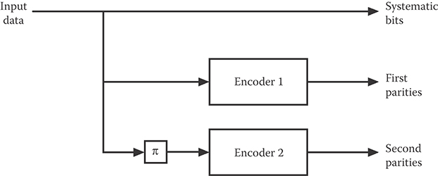
FIGURE 6.6 The structure of a turbo encoder.

FIGURE 6.7 The turbo encoder from the 1993 ICC paper [10].
A decoder for such a turbo code is shown in Figure 6.8. The two constituent decoders correspond to the two constituent encoders, and they are used iteratively. Each decoder has three inputs—(1) the received channel values corresponding to the systematic (data) bits; (2) the received channel values corresponding to the parity (redundant) bits; and (3) a priori values for the systematic bits. The a priori values represent the initial probabilities assigned to the systematic bits by the decoder, and they are provided in the iterative framework by the other decoder. Heuristically, each decoder is provided with the channel values it needs plus a “first estimate” of the data—that is, for each systematic bit, a probability that that bit is “1.” The decoder then produces its own estimate of the data probabilities and passes them on to the other decoder—which uses them as its “first estimate.” In this way, the two decoders (ideally) make increasingly better estimates of the data.
The algorithm used by each decoder is the Bahl-Cocke-Jelinek-Raviv (BCJR) algorithm [14], a maximum a posteriori (MAP) decoding algorithm for convolutional codes. Unlike ML decoding, in which noisy values y are observed and the estimate of the data x is the value maximizing p(y|x), a MAP decoder observes y and chooses as its estimate of x the value maximizing p(x|y); such a decoder requires not only a probabilistic description of the channel (which is all that is required for an ML decoder) but also the a priori probabilities on x—something that, in a turbo decoder, is provided by the partner decoder.
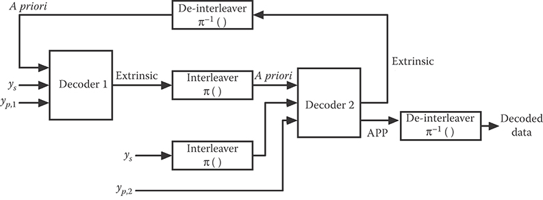
FIGURE 6.8 The structure of a turbo decoder. Here, ys indicates the received systematic values while yp,1 and yp,2 represent the received values corresponding to the first and second parity sequences, respectively.
Regarding the “first estimates” that each BCJR decoder produces (and that are used by the other decoder as a priori probabilities): These are labeled “Extrinsic” in Figure 6.8, and they must be computed in a way that removes (to the extent possible) the transfer of information to a decoder that is already using that information. As noted above, each decoder uses three inputs: systematic values, parity values, and a priori values. However, the other decoder already has access to two of those—the systematic values and the a priori values (which were produced by the other decoder as extrinsic information). Therefore, the effect of the systematic values and the a priori values must be removed from each decoder's “first estimate” before it is passed as extrinsic information to the other decoder. (For details on how this is accomplished, see, for example, [15] or [16].)
The algorithm stops either after a maximum number of iterations or when some “stopping condition” indicates to the decoder that the data have been correctly decoded. At that point, Decoder 2 produces its estimate of the data—and it does so without removing the effects of the systematic and a priori information as it does when passing extrinsic information. That is, Decoder 2 bases its final decisions on the a posteriori probabilities (APP) it computes for each systematic bit.
The performance of the 1993 ICC turbo code is shown in Figure 6.9. The improvement in performance as the number of iterations increases is vast; after only 18 iterations, a BER of 10−5 is obtained at a signal-to-noise ratio of only 0.7 dB—just a half dB above the limit implied by the capacity theorem for BPSK-modulated AWGN channels. Also notable is the “error floor”—the sharp reduction in the slope of the BER curve at BER values below 10−5. This phenomenon had not been observed with conventional, “pre-turbo” codes and was not initially understood by early turbo researchers. Subsequent research showed that the impressive “waterfall” performance of turbo codes is due to “spectral thinning”—that is, a reduction in the multiplicity of low-weight turbo codewords—while the error floor is due to the (relatively small) minimum distance of turbo codes.
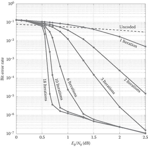
FIGURE 6.9 Performance of the rate-1/2 turbo code from Figure 6.6 assuming BPSK and additive white Gaussian noise.
Turbo codes represented a breakthrough in channel coding. Their startling performance demonstrated that the lessons of Shannon—that good codes should have long blocklengths and appear “random”—are still valid, but it also provided a new insight: That very long codes could be made practical by employing suboptimal iterative decoding techniques. All these lessons were present in the next coding “breakthrough”—low-density parity check (LDPC) codes.
6.5 Low-Density Parity Check Codes
LDPC codes were originally proposed by Dr. Robert Gallagher in the early 1960s [17], but it took more than 30 years—and the maturation of high-speed digital processing technology—for them to be recognized as a practical and powerful solution for many channel coding applications. Indeed, it was only in the aftermath of the discovery of turbo codes that the key elements of LDPC codes—long, random-like codewords made practical by an iterative decoding algorithm—were “rediscovered” and fully appreciated [18].
LDPC codes are block codes with a parity check matrix with a “low density” of ones—that is, relatively few ones. While there is no precise definition of what constitutes “low density”—typically, we take it to mean that the fractions of nonzero components in each row and each column are very small—the decoder complexity increases with the number of ones in the parity check matrix, so keeping the density of ones low is what makes LDPC codes practical.
As a simple example, consider the parity check matrix given by
(This matrix actually contains a relatively high density of ones, but it suffices to introduce the necessary terminology and concepts.)
The above parity check matrix illustrates a particular kind of LDPC code, called a regular LDPC code, because every row of the matrix and every column of the matrix contains the same number of ones. An (wc, wr) regular LDPC code is one for which the associated parity check matrix has wc ones in every column and wr ones in every row; thus, each code bit is involved in wc parity constraints and each parity constraint involves wr bits. It is easy to show that the rate R of an (wc, wr) LDPC code satisfies , where the quantity is called the design rate of an (wc, wr) LDPC code.
Associated with an LDPC code is a Tanner graph with two classes of nodes—check nodes and bit nodes; if the parity check matrix is m rows by n columns, then there are m check nodes (one for each parity check) and n bit nodes (one for each codeword bit) in the graph. An edge connects a check node with a bit node if and only if the bit participates in the associated parity check. The Tanner graph for the (2,4) regular LDPC code with parity check matrix H above is shown in Figure 6.10.
The significance of the Tanner graph is that it provides a “map” to the decoding algorithm that is typically used with LDPC codes—an algorithm called belief propagation or message passing. The details of the belief propagation algorithm can be found in any textbook on coding theory (e.g., [15,19]), but what follows is a brief overview.
The decoding algorithm is iterative, with each iteration consisting of two phases: In the first phase of an iteration, every bit node sends a “message” to every check node connected to the bit node via the Tanner graph; in the second phase, every check node similarly sends a message to each of the bit nodes to which it (the check node) is connected.

FIGURE 6.10 The bipartite graph for the (2,4)-regular LDPC code with parity check matrix given by H.
The messages passed from bit nodes to check nodes and from check nodes to bit nodes are called extrinsic information—“extrinsic” meaning that we do not pass to a node information that recently originated at that node.
Let qij denote a message passed from bit node i to check node j in a given round. Then, qij is the probability that the transmitted bit value associated with node i is “1,” given the received channel value and given all of the extrinsic information that was passed to bit node i in the previous iteration, with the exception of the extrinsic information that was passed to bit node i from check node j.
Let rji denote a message passed from check node j to bit node i. Then, rji is the probability that the parity check constraint described by check node j is satisfied, given that the transmitted bit value associated with node i is “1” and given all the extrinsic information passed to check node j from the other bit nodes (except for bit node i) in the previous round.
At the end of each iteration, the APP distribution for each bit node can be computed based on the associated channel output value as well as the messages passed to the node during that iteration. An estimate for each bit can be made at that point based on the APP value—that is, an estimate of “1” if that is the more likely value, an estimate of “0” otherwise.
The algorithm continues until either a fixed number of iterations have been completed or some “stopping condition” has been met—for example, if the hard estimates produced by the APP distributions at the end of an iteration satisfy all the parity constraints required by the code.
Figure 6.11 shows the dependencies of messages flowing into and out of a check node f0; in keeping with the notion that only “extrinsic” information is passed to a node, the message that f0 sends to X0 depends on the messages f0 received from X1, X2, and X3 but not X0—and similarly for the other messages passed by f0. Similarly, Figure 6.12 shows the dependencies of messages flowing into and out of bit node X0; here, Y0 corresponds to the matched-filter channel output corresponding to the value of X0.

FIGURE 6.11 The dependencies of messages passed to and from check node f0 in message-passing decoding of LDPC codes.

FIGURE 6.12 The dependencies of messages passed to and from a bit node X0 in message-passing decoding of LDPC codes.
The algorithm as outlined above involves the passing of messages that represent probabilities, or likelihood values; in practice, it is common to carry out the algorithm in the log domain, so the messages become log-likelihood ratios (LLRs) that are either positive or negative—that is, the sign of the LLR indicates whether the associated random variable is more likely to be “1” or “0,” and the magnitude of the LLR reflects the confidence of that assertion. Executing the algorithm in the log domain has the advantage of turning costly multiplications into less costly additions and also enhancing numerical stability.
Figure 6.13 demonstrates the performance of three different (6,3)-regular LDPC codes (each of design rate 0.5) over a BPSK-modulated AWGN channel. The advantage of increasing the code's blocklength is apparent; for a bit error rate of 10−5, increasing the blocklength from n = 2000 to n = 200,000 provides almost a full decibel of coding gain.

FIGURE 6.13 The performance of a (3,6) regular randomly designed LDPC code over a BPSK-modulated additive white Gaussian channel for blocklengths of n = 2000, 10,000, and 200,000 bits.
The results in Figure 6.13 show LDPC performance that is still significantly worse than what is promised by Shannon and information theory; the capacity of the BPSK-modulated AWGN channel tells us that there exists a rate-1/2 code that can perform arbitrarily well at Eb/N0 = 0.184 dB—more than a full dB less than the SNR required for the n = 200,000 LDPC code to attain a bit error rate of 10−5. To get good performance at lower SNR values requires the use of irregular LDPC codes—that is, codes with parity check matrices with a nonconstant number of ones in every row and column; indeed, by optimizing the degree profiles that characterize the densities of ones in the matrix's rows and columns, it is possible to get good performance within a few hundredths of a dB from the limit imposed by capacity [20].
6.6 Coding and Bandwidth-Efficient Modulation
The bandwidth of a communication channel imposes limits on how rapidly one can signal over the channel. Specifically, the results of Nyquist dictate that it is impossible to transmit more than W two-dimensional symbols per second over a W Hz bandpass channel without incurring intersymbol interference (ISI) at the receiver.
While Nyquist tells us we cannot send more than W symbols per second, it is still possible to improve the data rate over a W Hz channel by conveying more information with each symbol—that is, by using bandwidth-efficient modulation. In uncoded transmission, a symbol constellation with M = 2b symbols conveys b bits with every symbol; Figure 6.14 shows symbol constellations with M = 4, 8, and 16 symbols, corresponding to b = 2, 3, and 4 bits per symbol; these constellations are called quaternary phase-shift keying (QPSK), octal phase-shift keying (8-PSK), and 16-ary quadrature amplitude modulation (16-QAM).
A brief explanation of what these constellations represent: Each symbol has an associated b-bit label; therefore, the transmission of each symbol is equivalent to the transmission of b bits. But what does it mean to “transmit” a symbol? Think of the constellations in Figure 6.14 as lying in the complex plane, so the “x-coordinate” of each symbol represents its real part and the “y-coordinate” its imaginary part. Then, to transmit the sequence of symbols [s0, s1, s2, …] means to transmit the signal c(t), where
The orthogonality of the two sinusoids creates, in essence, two channels; the in-phase channel that carries the real part of each transmitted symbol and the quadrature channel that carries the imaginary part. The pulse p(t) is used to shape the spectrum of the transmitted signal, and these pulses are transmitted every Ts seconds, each pulse weighted by the appropriate symbol coordinate. Raised cosine pulses are often used in this context; a raised cosine pulse with rolloff parameter α (0 ≤ α ≤ 1) results in a transmitted signal with a bandwidth of (1 + α)/Ts Hz. Thus, uncoded M-ary transmission provides a bandwidth efficiency of γ = log2(M)/(1 + α) bits/s/Hz.
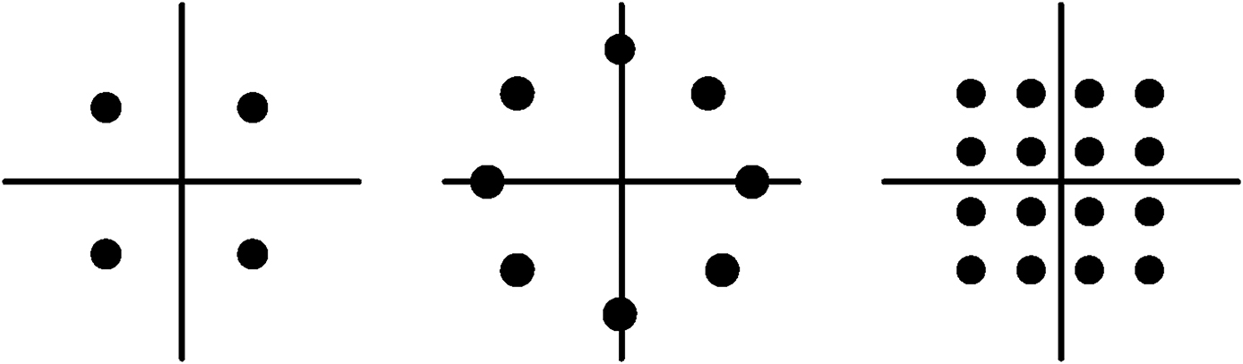
FIGURE 6.14 Three constellations for bandwidth-efficient modulation: QPSK, 8-PSK, and 16-QAM.
While channel coding for power-limited applications (e.g., space communications) yielded useful results as early as the mid-1960s, the application of channel coding to bandlimited environments (such as the telephone channel) came much later. The reason: the straightforward application of binary codes to larger, “denser” symbol constellations—that is, by designing good binary codes and then mapping them via Gray mapping* to the larger constellation—yielded relatively poor results.
With hindsight, the reason for the disappointing performance is obvious. The performance of a digital communication system is, to first order, determined by how “far apart” two different, valid transmitted symbol sequences are required to be; the more “unlike” two sequences are from one another, the less likely the receiver is to mistake one for the other. Here, the “distance” of one sequence from another is given by the square root of the cumulative squared Euclidean distance between the symbols—that is, the distance between the sequence of symbols [s0, s1, s2, …] and the sequence [r0, r1, r2, …] is . However, encoding data with good binary codes and then “throwing the encoded bits over a wall” to be modulated does not result in a system with good Euclidean distance properties.
In the late 1970s, Gottfried Ungerboeck [21] of IBM unveiled trellis coded modulation (TCM), a technique for jointly designing the coding and modulation functions to enhance Euclidean distance properties; TCM is still employed in wireline and wireless systems today. Another approach to bandwidth-efficient coding, bit-interleaved coded modulation (BICM), was originally developed to improve performance over fading (mobile) communication channels [22] but has since, with the advent of capacity-approaching codes such as turbo and LDPC codes, been shown to be useful in a variety of applications. The next two subsections describe TCM and BICM.
6.6.1 Trellis-Coded Modulation
TCM is best explained via a (now classic) example. Suppose one wishes to convey two information bits per transmitted symbol—a goal that is realizable with uncoded transmission using QPSK modulation. TCM teaches that, to apply coding to such a system, one doubles the constellation size—to 8-PSK—and then uses the structure of a convolutional encoder to ensure that only certain sequences are valid and can thus be transmitted.
This approach is illustrated in Figure 6.15. Two information bits are passed through a rate-2/3 convolutional encoder to produce the three bits [y2y1y0]. This convolutional encoder is not “good” in the sense that it has a large free distance; indeed, its free distance is trivially one. Rather, the output of the encoder is interpreted as the label of the transmitted symbol, and the combination of the encoder with the “natural” (rather than Gray) mapping produces an encoder-plus-modulator with better Euclidean distance properties than uncoded QPSK. Specifically, this scheme provides an asymptotic (high-SNR) coding gain of approximately 3 dB in AWGN compared to uncoded QPSK, meaning that the coded system need transmit only half as much power as the uncoded system and still have the same performance.
To understand the TCM encoder in Figure 6.15, it is informative to look at the state transition diagram. Because the encoder has ν = 2 memory elements, this is a four-state encoder. Moreover, because only one of the two input bits is passed through the encoder—the other is uncoded—there are parallel transitions between states. For example, if the encoder is in state “00” then an input of either “01” or “11” will cause a transition to state “10”; because the first bit is uncoded, it has no effect on the state transition. Finally, observe that the two transmitted symbols corresponding to these two parallel transitions—symbols S2 and S6—are maximally far apart.
These observations lead to an illuminating interpretation of the encoder in Figure 6.15: The encoded bits [y1y0] select a sequence of subsets of the symbol constellation—in this example, there are four such subsets: {s0,s4}, {s1,s5}, {s2,s6}, and {s3,s7}—and then the uncoded bit is used to select one of the symbols from the subset. Thereby, the sequence of two-bit inputs selects a sequence of 8-PSK symbols that are transmitted.
*In Gray mapping, labels are assigned to two-dimensional symbols so that adjacent symbols have labels that differ in a single bit. In this way, the most common symbol detection errors result in a single bit error.
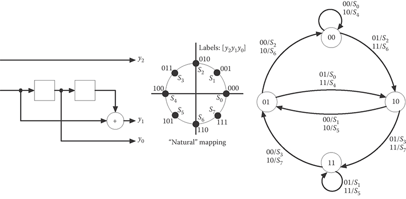
FIGURE 6.15 A trellis-coded modulation (TCM) scheme employing 8-PSK to convey two information bits per symbol.
This approach is generalized in Figure 6.16 to describe a system in which k information bits are conveyed with every transmission of a symbol from a constellation with 2k+1 elements—i.e., the constellation size is doubled over what is required for uncoded transmission. In this figure, k data bits enter the encoder during each symbol period; m of them are coded while k–m of them are uncoded. The m coded bits are passed through a rate-m/(m + 1) convolutional encoder to produce m + 1 bits that form part of the label of the transmitted codeword; the k–m uncoded bits form the rest of the k + 1-bit label. In this way, the output of the convolutional encoder selects a sequence of constellation subsets—there are 2m+1 such subsets, and they each contain k–m symbols—while the uncoded bits select the transmitted symbol from each subset thus selected. (Applying this notation to the example in Figure 6.15, we have k = 2 and m = 1.)
The 2m+1 subsets (each with 2k–m symbols) should be designed to be as “sparse” as possible; the minimum Euclidean distance between symbols in each subset should be maximized. This is because two information sequences that differ in a single uncoded bit will be encoded to symbol sequences that are at least dmin,uncoded apart, where dmin,uncoded is the minimum Euclidean distance within a (sparse) subset. On the other hand, two information sequences that differ in coded bit(s) will benefit from the structure of the convolutional encoder; the convolutional encoder guarantees that the sequence of (partial) labels it produces will yield a sequence of subsets that are sufficiently different to guarantee a cumulative Euclidean distance of dmin,coded. Thus, the overall scheme produces a guaranteed minimum Euclidean difference of dmin = min{dmin,coded, dmin,uncoded} in the two sequences of transmitted symbols associated with two different information sequences.

FIGURE 6.16 A block diagram of a generic TCM encoder.
TCM has been widely extended beyond the simple approach outlined here [15,16]. Examples of those extensions include:
The design of multidimensional trellis codes, in which the symbol constellation is not two-dimensional but rather 2M-dimensional for some integer M > 1. The 2M-dimensional space is obtained by concatenating M successive two-dimensional spaces created by the in-phase/quadrature representation of M symbol intervals. The advantage of higher-dimensional codes comes from the fact that it is possible to more efficiently “pack” symbols in higher dimensions.
The design of rotationally invariant trellis codes, which enable the receiver to recover the transmitted data even when the symbol constellation is rotated—a phenomenon that occurs when the receiver loses carrier synchronization and is unable to acquire an absolute phase reference.
6.6.2 Bit-Interleaved Coded Modulation
While TCM employs an integrated approach to coding and modulation, BICM takes a partitioned approach—but with the addition of a bit-interleaver between the encoder and the modulator.
In an early paper by Zehavi [22], BICM was motivated by the fading present in mobile communication channels. In the fully interleaved Rayleigh fading channel, it is assumed that each transmitted symbol is affected independently by Raleigh fading; this is quite different from the block Rayleigh fading channel in which the fading is assumed to be (approximately) constant over some specified blocklength, typically determined by vehicle speed and carrier frequency.* The performance of a coded digital communication system over the fully interleaved Rayleigh fading channel is affected most strongly by its diversity order—that is, by the minimum number of distinct modulation symbols between two valid transmitted sequences; this is quite different from the cumulative squared Euclidean distance metric that determines performance over a nonfading AWGN channel—and which motivated TCM. Zehavi's approach, illustrated in Figure 6.17 with a rate-2/3 convolutional code, was to carry out “bit-interleaving” between the encoder and the decoder to “spread out” the bits so that every bit-difference in the convolutional encoder's output produced exactly one corresponding symbol-difference in the transmitted sequence; this leads to a diversity order equal to the minimum Hamming distance of the convolutional encoder—the optimal value.
Subsequent research on BICM [23] indicated that very little capacity is lost (for both fading and AWGN channels) by restricting the encoder to one of the type from [22]—that is, by using bit interleaving to create independent, binary-input equivalent channels and then applying capacity-approaching codes to those channels. This realization, coupled with the concurrent development of capacity-approaching binary codes such as LDPC and turbo codes, has led to the widespread adoption of the BICM architecture—a binary encoder followed by a bit interleaver followed by a dense Gray-mapped symbol constellation—for bandwidth-efficient communication.
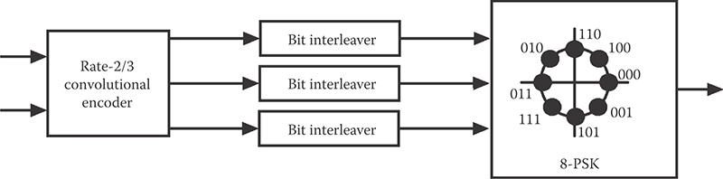
FIGURE 6.17 Block diagram of the rate-2/3 8-PSK BICM encoder. (From Zehavi, E., IEEE Transactions on Communications, 40(5), 873–884, 1992.)
*The fully interleaved Rayleigh fading channel can be realized by symbol-interleaving a block-wise (or correlated) fading channel to sufficient depth that the fades from one symbol to the next appear independent.
6.7 Automatic Repeat Request
All the approaches to error control described in this chapter up to this point have been examples of FEC. This means that the redundancy incorporated into the transmitted signal is designed to provide enough robustness against channel noise that the information-bearing sequence can be recovered at the receiver well enough to meet the application's requirements without any retransmissions.
For some applications, it is wasteful to provide such a high level of robustness because the channel conditions are usually so benign that the redundancy is unneeded. For such applications, when a “reverse channel”—a channel from the receiver to the transmitter—is available, an ARQ approach is appropriate.
In an ARQ protocol, the receiver does not attempt to recover the encoded data in the presence of corruption; rather, it simply detects the corruption and, when upon finding it, requests that the data be retransmitted. Thus, an ARQ protocol requires two elements: a means for error detection and a retransmission strategy.
Error detection is typically carried out using an error-detecting code. A class of codes commonly used for this purpose is the cyclic redundancy check (CRC) codes. CRC codes are (n,k) block codes—that is, codes with k data bits and n-k redundant bits—wherein the redundancy is used to only detect the presence of errors rather than correct them, as described in Section 6.2. For instance, CRC-12 is a code that adds 12 bits of redundancy to a data packet to create an n-bit codeword, where n ≤ 2047; these 12 bits of redundancy guarantee that 12 different parity constraints are satisfied across the codeword. This code has a minimum distance of dmin = 4, so, provided no more than three bit errors occur in the codeword, the resulting syndrome (see Section 6.2) will be nonzero, flagging a corrupted packet.
A wide variety of CRC codes are used in mobile communication standards. For example, the 3GPP cellular standard alone employs four different CRC codes—codes with three bits of redundancy, six bits of redundancy, eight bits, and fourteen bits—in its various modes.
Retransmission strategies require that the receiver informs the transmitter whether or not it has reliably received a particular packet or frame*; this is done by transmitting an “ACK” (a positive acknowledgment for an apparently uncorrupted frame) or a “NACK” (a negative acknowledgement for a corrupt frame). The transmitted frames typically include a header that contains a packet identification number; these ID numbers allow the receiver to indicate which frames have (and have not) been reliably received. Moreover, frames that have been neither ACKed nor NACKed within a specified “timeout” duration are treated as if they were negatively acknowledged.
Retransmission strategies come in at least three different flavors, corresponding to different trade-offs between complexity and efficiency.
Stop-and-Wait is the simplest retransmission strategy. It requires that a transmitter, upon sending a frame, wait until that frame is acknowledged before it sends (or resends) another. Thus, the protocol proceeds in a “ping pong” fashion with the transmitter and receiver alternately sending frames and acknowledgments (see Figure 6.18). Stop-and-Wait thus does not require a full-duplex channel—that is, it does not require simultaneous transmission in each direction—and, compared with more sophisticated approaches, it requires minimal storage and processing at both the transmitter and the receiver. However, this simplicity comes at a cost in throughput; because most channels are in fact full-duplex and Stop-and-Wait does not exploit this capability, the transmitter is sitting idle, waiting for acknowledgments, when it could be formatting and transmitting additional frames.
*In this chapter, we use the terms “packet” and “frame” interchangeably. Both terms refer to a data unit that typically includes user-supplied “payload” data as well as CRC redundancy and an identification number.

FIGURE 6.18 Timeline for a Stop-and-Wait ARQ protocol.
Go-Back-N is a retransmission strategy designed to address the inefficiency of Stop-and-Wait. In a communication link implementing the Go-Back-N strategy, the transmitter does not have to wait for a request before sending another packet. Rather, the transmitter is permitted to send all of the packets in a “window” maintained at the transmitter. When the first (earliest) packet in the window is ACKed, the transmitter “slides” the window one position, dropping the acknowledged packet and adding a new one which it then transmits; conversely, if a NAK is received for that first packet in the window, the transmitter “backs up” and resends all the packets in the window, beginning with the corrupt packet.
More specifically, suppose that the transmitter has received an ACK for Packet i. Then, under the Go-Back-N protocol, the transmitter may send Packets i + 1 through i + N without receiving another ACK; however, the transmitter must receive an ACK for Packet i + 1 before transmitting Packet i + N + 1 (see Figure 6.19).
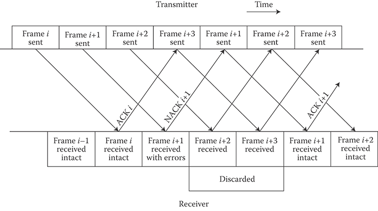
FIGURE 6.19 Timeline for a Go-Back-N ARQ protocol. This timeline assumes N ≥ 3.
Go-Back-N is often referred to as a sliding window protocol because the transmitter maintains a sliding window of “active” frames—that is, up to N frames that have been transmitted but have not yet been acknowledged. It should be clear that the Stop-and-Wait strategy is simply a Go-Back-1 strategy.
Finally, the Go-Back-N protocol is clearly still not as efficient as it could be; when a frame is corrupted under the Go-Back-N protocol, all the frames that were transmitted after the bad frame was sent and before it was negatively acknowledged must be retransmitted as well—as many as N − 1 frames in addition to the corrupt frame. These discarded frames may have, in fact, been received error-free; they are discarded only because they followed too closely on the heels of a corrupt frame.
Selective-Repeat ARQ overcomes this inefficiency. In the Select-Repeat protocol, the transmitter does not retransmit the contents of the entire window when an NAK is received; rather, the transmitter resends only the frame “selected” as corrupt by the receiver. Selective-Repeat is typically implemented as a sliding window protocol, just like Go-Back-N. This means that, when Frame i is ACKed, Frames i + 1 through i + N (but not Frame i + N + 1) may be transmitted before Frame i + 1 is positively acknowledged. Once Frame i + 1 is ACKed, all the “oldest” frames in the window that have been positively acknowledged are considered complete and are shifted out of the window; the same number of new frames are shifted into the window and are transmitted.
This process is illustrated in Figure 6.20. Here, Frame i is received intact and Frame i + 1 is corrupt; however, in the Selective-Repeat strategy, Frames i + 2 and i + 3—the two frames sent after Frame i + 1 was sent but before it was negatively acknowledged—are not discarded at the receiver (and resent by the transmitter) but instead are accepted, assuming they are not corrupt.
Finally, it should be noted that hybrid ARQ (HARQ) schemes [24,25]—containing elements of both FEC and ARQ—have also found applications in mobile communication systems. Hybrid ARQ schemes employ FEC codes to make a “first attempt” to decode a frame; if that attempt is unsuccessful, then some kind of retransmission is employed. Hybrid ARQ schemes are typically classified into one of two approaches:
In a type-I hybrid ARQ system, a conventional FEC code (of the type described in Sections 6.2–6.6) is used in each frame. If the decoder can successfully recover the frame, then it does so. If the decoder cannot successfully recover the frame—something typically ascertained by using an “outer” error detection code that checks the results of the “inner” FEC code—then the receiver requests a retransmission of that same frame.
In a type-II hybrid system, what is retransmitted is not a copy of the same (encoded) frame that failed to decode on the first attempt, but rather additional redundant parity check bits for the same data. In this way, the receiver can observe a single (noisy) codeword from a longer, more powerful code spread out over two frames.

FIGURE 6.20 Timeline for a Selective-Repeat ARQ protocol.
References
1. C. E. Shannon, A mathematical theory of communication, Bell System Technical Journal, July–October, 1948, pp. 379–423, 623–665.
2. M. J. E. Golay, Notes on digital coding, Proceedings of the IRE, 37, 657, 1949.
3. R. W. Hamming, Error detecting and error correcting codes, Bell System Technical Journal, 29, 147–160, 1950.
4. A. Hocquenghem, Codes correcteurs d'Erreurs, Chiffres, 2, 147–156, 1959.
5. R. C. Bose and D. K. Ray-Chaudhuri, On a class of error correcting binary group codes, Information and Control, 3, 68–79, 1960.
6. I. S. Reed and G. Solomon, Polynomial codes over certain finite fields, Journal of the Society for Industrial and Applied Mathematics, 8, 300–304, 1960.
7. John G. Proakis, Digital Communications, 4th edition, McGraw-Hill, New York, NY, 2001.
8. V. Guruswami and A. Vardy, Maximum likelihood decoding of Reed-Solomon codes is NP-hard, IEEE Transactions on Information Theory, 51(7), 2249–2256, 2005.
9. J. Jing and K. Narayanan, Algebraic soft-decision decoding of Reed-Solomon codes using bit-level soft information, IEEE Transactions on Information Theory, 54(9), 3907–3928, 2008.
10. P. Elias, Coding for noisy channels, IRE Convention Record, 3, part 4, 37–46, 1955.
11. A. Viterbi, Error bounds for convolutional codes and an asymptotically optimum decoding algorithm, IEEE Transactions on Information Theory, IT-13, 260–269, 1967.
12. C. Berrou, A. Glavieux, and P. Thitimajshima, Near Shannon limit error-correcting coding and decoding: Turbo codes, Proceedings of the 1993 International Conference on Communications, Geneva, Switzerland, pp. 1064–1070.
13. C. Berrou and A. Glavieux, Near optimum error correcting coding and decoding: Turbo codes, IEEE Transactions on Communications, 44(10), 1261–1271, 1996.
14. L. Bahl, J. Cocke, F. Jelinek, and J. Raviv, Optimal decoding of linear codes for minimizing symbol error rate, IEEE Transactions on Information Theory, IT-20(2), 284–287, 1974.
15. S. Lin and D. J. Costello, Jr., Error Control Coding, 2nd edition, Pearson Prentice-Hall, Upper Saddle River, NJ, 2004.
16. T. Moon, Error Correction Coding, Wiley-Interscience, Hoboken, NJ, 2005.
17. Robert G. Gallager, Low-Density Parity-Check Codes, MIT Press, Cambridge, MA, 1963.
18. D. J. C. MacKay and R. M. Neal, Near shannon limit performance of low density parity check codes, Electronic Letters, 32(18), 457–458, 1996.
19. T. Richardson and R. Urbanke, Modern Coding Theory, Cambridge University Press, New York, NY, 2008.
20. S.-Y. Chung, G. D. Forney, T. Richardson, and R. Urbanke, On the design of low-density parity check codes within 0.0045 dB of the Shannon limit, IEEE Communications Letters, 5(2), 58–60, 2001.
21. G. Ungerboeck, Channel coding with multilevel/phase signals, IEEE Transactions on Information Theory, 28(1), 55–67, 1982.
22. E. Zehavi, 8-PSK Trellis’ codes for a Rayleigh channel, IEEE Transactions on Communications, 40(5), 873–884, 1992.
23. G. Caire, G. Taricco, and E. Biglieri, Bit-interleaved coded modulation, IEEE Transactions on Information Theory, 44(3), 927–946, 1998.
24. S. Lin, D. Costello, Jr., and M. Miller, Automatic repeat request error control schemes, IEEE Communications Magazine, December, 5–16, 1984.
25. L. Rasmussen and S. Wicker, The performance of type-I Trellis coded hybrid-ARQ protocols over AWGN and slowly fading channels, IEEE Transactions on Information Theory, March, 418–428, 1994.