
16
MIMO Systems for Diversity and Interference Mitigation
16.1 Advantages of Multiple Antennas Systems
Fading, Ergodic Capacity, Outage Capacity
Statistical MIMO Channel Models
Receive Diversity: SIMO with CSIR (MRC)
MISO and Diversity with CSIT (Beamforming)
MIMO Beamforming or Eigenbeamforming (Single Beam)
MISO and Diversity without CSIT, with CSIR (Alamouti's Scheme, Space–Time Codes)
Performance of Alamouti's Scheme
16.5 SIMO with Interference (Optimum Combining, MMSE Receivers)
16.1 Advantages of Multiple Antennas Systems
Systems with multiple antennas (see Figure 16.1) can exploit, besides the usual time and frequency, the spatial dimension, with large improvements in terms of diversity, interference mitigation, and throughput. For this reason, they are among the key technologies in modern wireless transmission systems [1–7]. Even in wired systems (such as in digital subscriber line (DSL) and in power line communication (PLC) systems), since cables usually contain multiple wires, the channel can be seen as a multiple-input multiple-output (MIMO). In the following, we will focus on MIMO wireless systems, but several of the described techniques can also be applied in wired systems.
The advantages of multiple antennas can be summarized as follows:
Array gain
This is the increase in the average signal-to-noise ratio (SNR) at the receiver due to coherent combination of signals. It can be obtained for both multiple transmit or multiple receive antennas, requiring channel state information at the transmitter (CSIT) or channel state information at the receiver (CSIR), respectively.
We define the array gain as
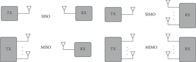
FIGURE 16.1 Multiple antenna systems: single-input single-output (SISO), single-input multiple-output (SIMO), multiple-input single-output (MISO), and multiple-input multiple-output (MIMO).
where SNRout and SNRSISO are the output SNR of the multiple antenna system and of the SISO system, respectively, and the average is taken with respect to fading (see following sections).
Diversity gain
In the presence of fading, the received power level can present large variations. Diversity is used to reduce the variations of the SNR level due to fading, by sending each information symbol through different channels with independent fading levels, and then combining the outputs. In a NT × NR MIMO channel, there are potentially NT · NR links. Spatial diversity can be obtained with multiple receiving antennas with CSIR (receive diversity), and with multiple transmit antennas (transmit diversity). Transmit diversity is possible both with CSIT (beamforming) and even in the absence of CSIT (Alamouti's code, space–time codes).
We can consider, as an indicator of the diversity order, the reduction of SNR variance:
Interference mitigation
Multiple antennas can be used as a spatial filter to reduce the power received from cochannel interfering sources. The enhanced robustness to cochannel interference increases the number of served users per unit area in wireless cellular systems.
Multipath multiplexing (spatial multiplexing) for high-throughput transmission
In MIMO channels with multipath, it is possible to transmit up to Nmin = min{NT,NR} “parallel” streams over the same band, with an increase of the link throughput. Multipath multiplexing, also called spatial multiplexing, is not possible for SIMO or MISO channels.
In this chapter, we describe systems with multiple antennas for diversity and interference mitigation. High-throughput MIMO systems are described in Chapter 17.
We start with the single-user scenario, and, for the sake of clarity, we focus on frequency-flat fading channels. The extension to wideband channel models is easy by assuming multicarrier transmission techniques, where the channel is frequency-flat for each subcarrier.
Throughout the chapter, vectors and matrices are indicated by bold, det A denotes the determinant of the matrix A, and ai,j is the (i,j)th element of A. The expectation operator is denoted by the superscript ()H denotes conjugation and transposition, I is the identity matrix, and tr{A} is the trace of A.
16.2 SISO Systems
16.2.1 System Model
Assume slowly varying frequency-flat wireless channels with additive white Gaussian noise (AWGN). For the SISO channel, this means that the discrete-time equivalent lowpass model (Figure 16.2) at time is
where are the received samples, are the transmitted symbols (e.g., belonging to M-ary quadrature amplitude modulation (M-QAM) or phase shift keying (PSK) constellations), are the noise samples, assumed independent, identically distributed (i.i.d.) circularly symmetric complex Gaussian (CSCG) random variables (r.v.s) with* . The channel gain is assumed constant over several symbols. Note that multiplication of the symbols x(k) by a complex gain h means that the constellation is scaled by |h| and rotated of an angle φ = arg h.
The SNR conditional to h is†
where Pt is the average transmitted power, and the Shannon capacity is
achieved when the symbols x(k) are i.i.d. CSCG. A different formula would hold when the symbols x(k) are constrained to belong to a specific constellation.
For ease of notation in the following we will drop, when possible, the time index k.
16.2.2 Fading, Ergodic Capacity, Outage Capacity
Assume now a fading channel, where h varies in time. In the so-called block fading channel (BFC) model, the channel h remains constant over a block of several symbols, taking i.i.d. values across different blocks. Thus, the fading process is specified by the block length (characterizing the time-correlation of the fading process) and by the distribution of the fading level within a block (e.g., h is a CSCG r.v. for a Rayleigh fading channel). In the following, we indicate with h(m) the fading level for the mth block.* The discrete-time process is ergodic (time averages equal ensemble averages) if the block duration is finite, and nonergodic if a realization is composed of just one block, that is, one fading level, lasting forever (in practice, for the duration of the communication).

FIGURE 16.2 Discrete-time equivalent lowpass representation of SISO.
*Note that circular symmetry implies zero mean, so .
†This SNR can be shown to be the ratio between the received energy per symbol and N0, conditional to a channel gain h, where N0 is the one-sided noise spectral density.
In Figure 16.3, we report a realization |h(m)|2Pt/σ2 for m = 0, … , 50 of a Rayleigh BFC (dashed curves). We set Pt/σ2 = 10, the channel gain has been normalized to give , giving the average signal-to-noise ratio . We observe that, due to Rayleigh fading, there are large fluctuations of the SNR values with m. The variations normalized to the average of the SNR are reported on the right plot. In the same figure, we show a realization of the SNR at the output of a SIMO system with NR = 8 antennas and maximal ratio combiner (MRC) receive diversity described in Section 16.4.1. We observe two effects of MRC: first, the average SNR is increased by a factor 8; second, the normalized SNR fluctuations are less severe. The first effect is called “array gain” (improvement in the average SNR). The second is called “diversity gain” (reduced variance of the normalized SNR as reported on the right plot).
*The block index m should not to be confused with the time index k. The two are coincident only when the block length is one symbol.
The variation of the SNR in time produces a variation of the link quality (throughput, error rate, delay, etc.). For example, we show in Figure 16.4 an example of C(h(m)) from Equation 16.3 for a realization of the time-discrete process h(m). Hereafter, we refer to Equation 16.3 as mutual information, since the concept of capacity requires some care (below). In the same figure, we report the capacity of the unfaded AWGN channel, log2(1 + SNR), and the average where the average is taken with respect to the distribution of h(m). The difference between the unfaded capacity and is relatively small (3.46 and 2.91 [bits/s/Hz], respectively). However, C(h(m)) shows large fluctuations around its average.
Recalling that the capacity is the maximum information rate that can be sent reliably across a noisy channel by using forward error correction (FEC) with sufficiently long codewords, we can distinguish two situations: the case where the codeword length is large with respect to a block (that we indicate as fast fading, or system with ideal time interleaving), and the case where the block duration is larger than the codeword length (slow fading, or system with no interleaving).
In this regard, is called ergodic capacity with channel unknown at the transmitter, and represents the information rate that a system with constant transmit power can achieve by using FEC when each codeword spans many fading blocks, that is, with ideal time interleaving. In this case, the fluctuations of the channel are somewhat averaged out by time interleaving.
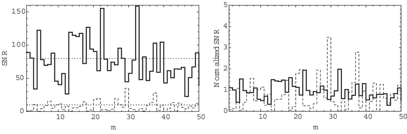
FIGURE 16.3 Example of behavior of the signal-to-noise ratio (left) and of the normalized output SNR defined as (right) for a system without diversity (dashed curves) and with diversity and array gain (solid curves). Rayleigh BFC model, m is the block index, average SNR per antenna equal to 10. Note that each block can consist of several thousands symbols. Red curve: SISO. Blue curve: SIMO MRC with NR = 8. The dotted curves on the left represent the average SNR. With MRC we have both an array gain (increase in the average SNR from 10 to 80) and diversity gain (a reduced variance of the normalized SNR as reported on the right).
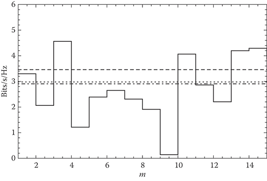
FIGURE 16.4 Example of behavior of C(h(m)) for the channel h(m), Rayleigh BFC model, average SNR equal to 10 dB, m is the block index. Note that each block can consist of several thousands symbols. Solid curve (3.46 [bits/s/Hz]): mutual information (16.3). Dashed curve: capacity for the unfaded AWGN. Dot-dashed curve (2.91 [bits/s/Hz]): mean value of Equation 16.3 with respect to the distribution of h (ergodic capacity with channel unknown at the transmitter). Dotted curve (2.98 [bits/s/Hz]): ergodic capacity with channel known at the transmitter, power, and rate time-adaptive system.
When the codeword length is of the order of the fading block (slow fading), and assuming the information rate R (information bits/s/Hz) at the channel input is constant, the mutual information (16.3) will be for some blocks smaller than R, and for some larger than R. From information theory we know that the codewords in the former case will not be correctly decoded,* while for the latter the codewords will be successfully decoded, provided a sufficiently powerful FEC coding scheme is adopted. We can therefore define the channel outage probability as follows:
which represents a lower bound on the codeword error rate for coded systems with information rate R at the input of a slow-fading channel without interleaving. We can also define the outage capacity at codeword error rate Ptarget as the value Rout to use at the channel input to guarantee a target outage probability Ptarget
and the resulting effective rate is Rout (1 − Pout(Rout)) (correctly received [information bits/s/Hz] over many fading blocks). This is sometimes called outage rate.
Assume now that the channel state h(m) is available at the transmitter side, a situation indicated as CSIT. In this case, a possibility, for the slow-fading channel case, is to change the information rate R(m) (information bits/s/Hz) for each block m, adapting its value below C(h(m)), so that the received codeword can be successfully decoded. The information rate is adapted by changing the FEC code rate and modulation format. In practice, a predefined set of couples (codes, modulation format) can be used to discretize the information rate. The transmitter then chooses the couple based on C(h(m)). Over a large number N of blocks the transferred rate achievable is bounded by which, for the law of large numbers, converges to . Thus, is also the achievable rate for a rate time-adaptive system.
*Recall that, for rates above capacity, the error probability goes exponentially to 1.
Still assuming CSIT, if we can also adapt the transmit power on a block-by-block bases, we could spend, for a given time-average power, more energy on the blocks with better SNR, and less on those with lower SNR, according to the water-filling principle. This power and rate time-adaptive system has a slightly larger achievable rate than the rate time-adaptive system, but with some additional practical issues due to the power variation with time.
For both rate time-adaptive and power and rate time-adaptive techniques, the information rate (i.e., number of information bits per block) change from block to block. For delay-sensitive applications this can be a problem, and constant rate solutions are preferable. For example, the transmit power can be varied to maintain a constant SNR at the receiver, and consequently a constant rate (like power control in cellular systems, also called channel inversion).
These considerations will be extended to MIMO channels in Chapter 17.
16.3 MIMO Channel Models
We here summarize some characteristics of MIMO channels [7–9]. Assuming a frequency-flat channel, matched filtering, and sampling with proper timing, the discrete-time equivalent lowpass model at time for MIMO channels is
where , xj(k) is the symbol transmitted at sample time k from the jth transmit antenna, the vector is the vector of the samples at the output of the NR antennas, and is a vector of noise samples, assumed i.i.d. CSCG r.v.s. The channel matrix has entries hi,j representing the complex gain from the jth transmit antenna to the ith receive antenna.
Important characteristics of the channel model (16.6) are the rank of the channel matrix* H (for a specific matrix) or the correlation among its elements (for statistical models). We will analyze below some specific situations.
16.3.1 MIMO Line-of-Sight Channel
Let us assume the transmission of a passband signal , where f0 is the carrier frequency and s(t) is the equivalent lowpass of . We assume that the signaling interval is T, which means that the variation rate of s(t) is approximately 1/T. A delay τ on the passband signal introduces a delay and a phase variation on the equivalent lowpass, since .
The MIMO channel with line-of-sight (LOS) propagation is depicted in Figure 16.5. We indicate as di,j and τi,j the path length and delay associated with the path from the jth transmit antenna to the ith receive antenna, respectively. We also indicate with the complex channel gain whose modulus is related to the path loss and antenna gains, and whose argument is related to the path delay. The equivalent lowpass of the signal at the output of the ith receive antenna is therefore
*Note that the rank of H is always limited by the minimum between NT and NR.
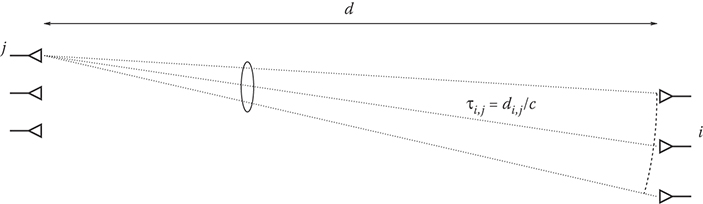
FIGURE 16.5 Geometry for a MIMO line of sight. The delay for the generic path is τi,j = di,j/c, where di,j is the path length and c is the light speed.
where ni(t) is the thermal noise. Although the path lengths di,j are, strictly speaking, different, if the distance d between the transmitter and the receiver is much greater than the antenna elements spacing, the difference among them is negligible and we can write . Therefore, in the above hypotheses, we can write
where the are all equal. Assuming matched filtering and sampling with proper timing, the discrete-time equivalent lowpass model at time is therefore given by Equation 16.6 where the channel matrix has entries hi,j which are practically identical, and has therefore rank 1. Thus, for MIMO LOS channels with link length d large compared to the antenna elements spacing, the channel model is given in Equation 16.6 where the matrix H can be considered rank 1.
16.3.2 MIMO with a Point Scatterer
Consider now the situation in Figure 16.6, where the emitted radiation is scattered by a single point scatter. We assume that all delay differences are small compared to the signaling interval T. Thus, the channel model is still of the form (16.6) but with a channel matrix , where h(TX→S) is the NT × 1 propagation vector from the transmitter to the scatterer, and h(S→RX) is the NR × 1 propagation vector from the scatterer to the receiver. These two vectors can be expressed precisely from the geometry depicted in Figure 16.6. From basic algebra, we know that, since H is the product of two vectors, it is rank 1. Thus, with one point scatterer, the channel matrix H in Equation 16.6 is rank 1.
16.3.3 MIMO with Multiple Scatterers
Assume now several point scatterers with delay differences which are small compared to the signaling interval T. Then, by the previous argument, the channel model is still of the form (16.6) with a channel matrix
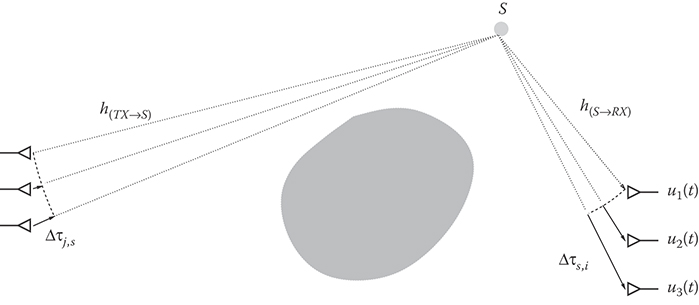
FIGURE 16.6 Geometry for propagation with a single point scatterer.
where , are the NT × 1 and NR × 1 propagation vectors for kth scatterer. From basic algebra, we thus obtain that the rank of H is at most equal to the number of scatterers (scatterers with the same direction of departure or of arrival will not increase the channel matrix rank). For a very large number of scatterers, the sum in Equation 16.9 can be thought of as an integral.
16.3.4 Statistical MIMO Channel Models
Consider now the ensemble of all possible channel matrices H, when the relative positions of the scatterers are subject to small random variations, due, for example, to movement of the transmitter, of the receiver, or of the environment. In this case the evolution of H with k is described by a discrete-time random process, where the elements of the channel matrix are randomly varying. The rate of variation of H depends on the rate of variation of the environment, that is, on the mobility of transmitter, receiver, and scatterers. The channel H at a given time k can be considered a random matrix, that is, a matrix with elements that are random variables, and a realization of it can be interpreted as the channel for a specific snapshot of the varying environment [10].
Let us consider a stationary channel, so that the first-order description of H(k) does not depend on k. If we assume that the randomly placed scatterers introduce delay differences which are small compared to the signaling interval T, the system model is still given by Equation 16.6, where H has elements hi,j described as random variables. When the number of independent scatterers is large, from the central limit theorem, the elements hi,j are complex Gaussian r.v.s, and their joint distribution can be given by specifying all mean values, , and all pairs correlation, that is, the matrix , where vec(H) is the (NT · NR) × 1 vector obtained by stacking the columns of H on top of one another.
Often, the correlation at the transmitter side (i.e., among the elements of a row of H) is the same for all rows, and the correlation at the receiver side (i.e., among the elements of a column of H) is the same for all columns. In this case, the correlation matrix can be factorized as where ⊗ denotes Kronecker product, and RT and RR describe the correlation at the transmitter and receiver side, respectively. This Kronecker model implies that the correlation at the receiver (transmitter) does not affect the spatial properties of the signals at the transmitter (receiver).
The spatial correlation is in general related to the angular distribution of the rays and the antenna elements spacing. Roughly speaking, many scatterers around the receiver (transmitter) give low correlation at the receiver (transmitter) side, while if all paths at one side arrive from a small angle, the correlation on that side is large, implying an overall rank-deficient channel.
For rich scattering environments with no dominant paths, one common model consists in assuming the elements hi,j as CSCG, implying (Rayleigh MIMO channels). Generally, if the spread of the angles of departure and of arrival are large,* the correlation is also small and the hi,j can be considered i.i.d. This is the Rayleigh uncorrelated MIMO channel model.
16.4 Diversity Techniques
16.4.1 Receive Diversity: SIMO with CSIR (MRC)
Consider the SIMO scheme in Figure 16.7. The NR-dimensional signal at the output of the receiving antennas at time k can be written as
where is a vector containing the complex gains between the transmit antenna and the NR receive antenna, is the transmitted symbol at time k, is the noise vector at time k with i.i.d. CSCG entries and covariance matrix .
Here, conditionally to hx(k), the vector y(k) is Gaussian, and the best linear estimate of the transmitted symbol is†
with weights
Note that Equation 16.12 requires that the channel gains (amplitude and phase) are known at the receiver. So, for each antenna element, we need a channel estimator (e.g., based on pilot symbols periodically embedded in the data symbols). Linear combining of the received signals with weights of the type w = Kh, as in Equation 16.12, with K an arbitrary constant, is called Maximal Ratio Combiner (MRC).‡ The SNR at the combiner output is
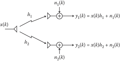
FIGURE 16.7 Discrete-time equivalent lowpass representation of a 1 × 2 SIMO.
*This condition in some particular cases is not sufficient. An example is the so-called keyhole channel, where, despite scattering, all paths are forced to pass through an intermediate point like in Figure 16.6; thus, as in Section 16.3.2, the overall channel matrix is rank 1 since it can be expressed as the product of two vectors.
†This estimate produces a sufficient statistic for the detection of the transmitted symbol and, as we will see later, is capacity-optimal.
‡It is easy to show that weights in the form w = Kh give the maximum SNR after the combiner.
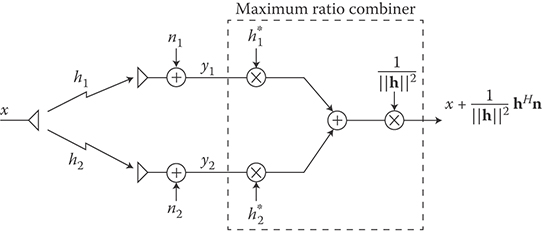
FIGURE 16.8 Implementation of MRC (time is dropped for ease of notation).
where Pt is the average transmitted power. It is easy to verify that, when the hi are i.i.d., the array gain is NR and the diversity order is also NR.
The implementation of MRC is sketched in Figure 16.8.
16.4.1.1 Optimality of MRC
For a given h, with MRC we have turned the SIMO into a SISO channel with capacity
This is also the capacity of the original SIMO (see Chapter 17); therefore, we can say that MRC is capacity-optimal for SIMO channels with perfect CSIR.
16.4.1.2 MRC in Fading Channels
Up to now we assumed a given channel h. Let us now assume slowly varying multipath propagation. Then, if for a time window of, let us say, a thousand symbols, there is a given h, for another window, due to the different combination of multipaths, there could be a different h. In other words, we assume to have a BFC, where the channel is constant for several symbols (a block), and varies from a block to another. So, if we focus on what happens to a block, we need to describe the first-order statistical variations of the channel, and consider h as a random vector with a given distribution.
For example, for the Rayleigh channel model, the elements of the vector h are CSCG. If the fading levels are uncorrelated from antenna to antenna, these elements are i.i.d., and the random variable is the sum of the modulus square of 2NR real i.i.d. Gaussian r.v.s.
The distribution of the sum of the squares of N i.i.d. zero-mean real Gaussian r.v.s is called central chi-square with N degrees of freedom and indicated as . Therefore, the distribution of is related to By using this distribution it results that, for Rayleigh fading channels where the fading is uncorrelated from antenna to antenna, the probability density function (p.d.f.) of the output SNR in Equation 16.13 results as

FIGURE 16.9 Performance of 1 × NR SIMO, MRC (so, with CSIR), Rayleigh fading, NR = 1,2,4,8 antennas, BPSK modulation. The same curves applies to NT × 1 MISO beamforming (so, with CSIT), with NT = 1,2,4,8, where the abscissa is .
where
can be interpreted as the average SNR per receiving antenna. This distribution can be used to evaluate the performance of digital modulation and coding schemes. For example, in Figure 16.9, the average bit error probability (BEP) for an uncorrelated Rayleigh fading SIMO channel with MRC, for a system using binary phase shift keying (BPSK) modulation is reported. As can be noticed, over Rayleigh uncorrelated channels, the BEP of uncoded systems with diversity order div has, for large SNR, a linear behavior in a log-log plot, with a slope of 10/div (dB/decade).
16.4.2 MISO and Diversity with CSIT (Beamforming)
Consider the MISO scheme in Figure 16.10, and assume that the transmitter knows perfectly the channel. The objective is to improve the performance by sending on the transmit antennas a linearly precoded version of the symbol x(k).
The weights α1, α2 must be designed to focus the transmitted energy toward the receiver, to produce the maximum SNR at the receive antenna. The power at the ith transmit antenna is , and we impose the normalization to have an average total transmitted power as for the single transmit antenna case.
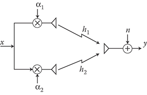
FIGURE 16.10 2 × 1 MISO beamforming.
The received signal is
It is easy to see that the best SNR for y(k) is obtained by choosing , where K is a normalization constant with . Taking K > 0 real (the phase of K can be included in the carrier phase), we have
The choice makes the signals at the receive antenna to add coherently, and the resulting SNR at the receiver is
which is exactly the same as for the MRC output (16.13).
This scheme can be called beamforming or eigenbeamforming and gives, for MISO with CSIT, exactly the same performance as for a SIMO MRC with CSIR (for the same total power Pt and channel gains hℓ). In particular, the array gain is NT and the diversity order is NT.
Different from MRC, here the transmitter must know the channel (amplitudes and phases for all hl). The ways to obtain this information are essentially two:
If the system adopts a time division duplex (TDD) technique, the channel estimated in reception (e.g., by using pilot symbols) can be used, for reciprocity, as an estimate of the channel in transmission (assuming the channel does not vary too fast).
In closed-loop systems, the receiver estimates the channel and sends the estimates back to the transmitter. This requires a feedback channel, with problems related to delays, quantization, and transmission errors.
16.4.2.1 Optimality of Beamforming for MISO
For a MISO with beamforming, the resulting end-to-end SISO has capacity given again by Equation 16.14, which is also the capacity of the original MISO assuming CSIT. Thus, beamforming is capacity-optimal for MISO with CSIT.
16.4.3 MIMO Beamforming or Eigenbeamforming (Single Beam)
The previous approach can be easily extended to the case when both the TX and the RX are equipped with multiple antenna (Figure 16.11). We call this MIMO beamforming or eigenbeamforming (single beam).
The received vector is
where . Since the last expression looks like Equation 16.10 for SIMO channels, we have that the optimum weights to use in reception are immediately given by the MRC principle as
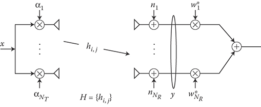
FIGURE 16.11 MIMO beamforming.
where K is an arbitrary constant and the corresponding SNR is
For the weights in transmission, we have to find the vector α, with , which maximizes Equation 16.22, that is, maximizing . Since HHH is Hermitian, we can use the spectral decomposition HHH = VΛVH, where the columns of the unitary matrix V are the eigenvectors of HHH, and Λ is diagonal with elements on the diagonal that are the eigenvalues of HHH. From linear algebra we recall that the vector α maximizing αHVΛVHα is the eigenvector of HHH corresponding to the largest eigenvalue λmax of HHH. In this case, it results as αHVΛVHα = λmax.
Thus, in summary
The optimum precoding vector αopt is the eigenvector of HHH corresponding to the largest eigenvalue λmax of HHH
The optimum combining vector is w = KHαopt
The resulting SNR at the output of the MIMO beamforming is
16.4.3.1 Optimality of Beamforming
The capacity of the end-to-end SISO obtained by the original MIMO with beamforming is therefore
It is interesting to note that, since , we have , where the equality is achieved when the channel matrix H has just one nonzero eigenvalue, that is, when it is rank 1. We will see that, for rank 1 channels, Equation 16.24 is indeed the capacity of the MIMO (see Chapter 17). Therefore, we can say that the scheme in Figure 16.11 is capacity-optimal for MIMO channels with rank 1 and CSIT (and sometimes also in other cases).
16.4.4 MISO and Diversity without CSIT, with CSIR (Alamouti's Scheme, Space–Time Codes)
We have seen that MISO beamforming requires CSIT, but is it possible to have transmit diversity without CSIT? Even looking at the simple 2 × 1 MISO it is quite clear that, if the TX does not know the channel, it is not possible by using a beamforming-like approach to find weights able to build distinct channels (and thus to provide diversity). However, it has been shown that by using, besides the spatial, the time dimension, it is actually possible to have transmit diversity even without CSIT. We discuss below the Alamouti's scheme for 2 × 1 MISO.
While in previous schemes we assumed to transmit a symbol x(k) (in a given time symbol T) and our aim was to recover that symbol, the key idea in space–time codes is to use time to build separable channels. So, assume we look at two consecutive symbols, x(k), x(k + 1), to be transmitted in two symbol periods. In a first symbol period T, we transmit x(k) on the first antenna and x(k + 1) on the second. In the second period, we transmit x*(k + 1) on the first antenna and −x*(k) on the second, as reported in Figure 16.12. The symbols are “precoded” by a factor to maintain .
At the receiver, the two samples received in the two consecutive time instants k, k + 1 are
By conjugating the second equation and defining , we can write
or, in short, , where

FIGURE 16.12 MISO Alamouti's scheme.
Now, by using time, with this construction we have in Equation 16.25 a virtual 2 × 2 MIMO. In principle, assuming the receiver knows h and therefore A (this means CSIR), the symbols x(k), x(k + 1) can be detected by using, for example, maximum likelihood (ML). However, here the situation is even simpler, since we observe that
that is, the matrix A is proportional to a unitary matrix. Therefore, if we compute we have
where it is easy to verify that the Gaussian vector has and , and is therefore statistically equivalent to the original noise n(k) = (n(k),n(k + 1))T. Therefore, we have the equivalent space–time channel
In other words, with this approach, the 2 × 1 MISO without CSIT can be interpreted as the SISO in Figure 16.13. In particular, we do not need to rethink to specific modulation and coding, since we can apply here all modulation and coding/decoding techniques for the SISO channel.
The virtual SISO channel obtained by the Alamouti's scheme has output SNR
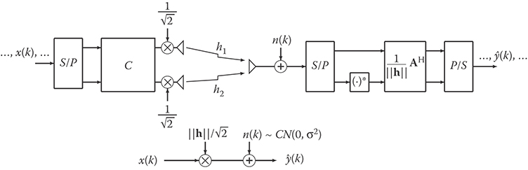
FIGURE 16.13 MISO Alamouti's scheme and its equivalent SISO. In the figure, is the encoder block, providing the two codewords C1 = (x(k), x*(k + 1)) and C2 = (x(k + 1), − x*(k)) to be transmitted over the first and second antenna, respectively. Note that these codewords are orthogonal for any x(k), x(k + 1).
Comparing this expression with Equation 16.19, we see that this 2 × 1 MISO scheme with no CSIT has the same performance of a 2 × 1 MISO with perfect CSIT and beamforming, except for a 3 dB loss (factor 2) in SNR. This loss is due to the lack of CSIT which does not allow precoding, like in beamforming, to have the coherent sum of signals at the receive antenna (here the weights in transmission are both equal to , meaning that the energy is transmitted uniformly in all directions).
In fact, the array gain is 1 (no array gain), while the diversity gain is NR = 2.
It is also easy to show that, for a 2 × NR MIMO Alamouti's scheme with channel matrix , we can replicate the scheme above for each receiving antenna (rows of H) and add the outputs. The SNR at the output of the combiner is the sum of the corresponding SNRs, that is,
From this expression, we see that the Alamouti's scheme uses the full 2 · NR diversity available.
This scheme, specifically designed for NT = 2, has the same spectral efficiency of a SISO, in the sense that two symbols are transmitted in two symbol periods. In this regard, the encoder used (see in Figure 16.13) is rate 1.
For NT > 2 it has been proved that similar orthogonal codes can be designed, but with rates strictly smaller than 1.
More in general, schemes like that in Figure 16.13, with suitable decoders, lead to the so-called space–time codes, where we can have block encoders (space–time block codes (STBC)), or trellis encoders (space–time trellis codes (STTC)). The Alamouti's scheme can be considered an STBC with NT = 2 and orthogonal codewords.
16.4.4.1 Optimality of the Alamouti's Scheme
The end-to-end capacity of the equivalent SISO obtained from the 2 × 1 MISO with the Alamouti's scheme is
which is also the capacity of the original MISO, assuming no CSIT (see Chapter 17). Therefore, the Alamouti's scheme is capacity-optimal for the 2 × 1 MISO with no CSIT.
For NR > 1, the capacity is
Similar to beamforming, since Equation 16.32 also represents the capacity for MIMO with rank 1 channels, we have that Alamouti's scheme for a generic 2 × NR MIMO with no CSIT is capacity-optimal if the channel matrix H is rank 1.
16.4.5 Performance of Alamouti's Scheme
The Alamouti's scheme can be used with coding and modulation designed for SISO channels, so its performances are those of a SISO system, with the SNR given by Equation 16.30. For example, in Figure 16.14, we report the BEP for uncoded Alamouti's scheme with M-QAM over a (2 × 2) MIMO Rayleigh uncorrelated fading channel with , as a function of Eb/N0 where Eb is the energy transmitted per information bit (see also Chapter 17).

FIGURE 16.14 BEP for uncoded Alamouti's scheme with M-QAM over a (2 × 2) MIMO Rayleigh uncorrelated fading channel with , as a function of Eb/N0, where Eb is the energy transmitted per bit. From left to right: M = 4,16,64,256 corresponding to 2,4,6,8 (bit/s/Hz).
16.5 SIMO with Interference (Optimum Combining, MMSE Receivers)
Multiple antennas have also the important advantage of mitigating cochannel interference. Consider for instance the situation in Figure 16.15, where the transmitted desired symbol x is received in the presence of cochannel interference due to one user transmitting on the same frequency band.
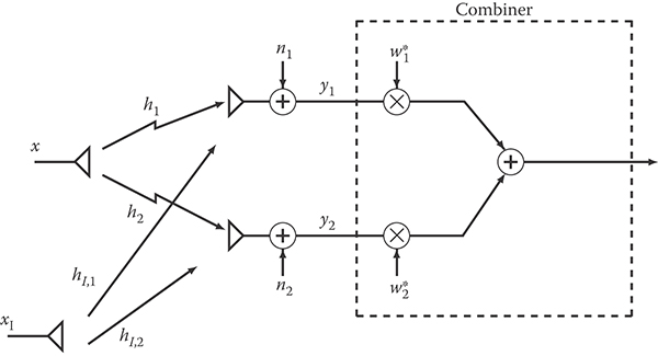
FIGURE 16.15 SIMO with interference.
The received vector is
where the time index has been omitted for ease of notation and hI, xI refers to the channel and symbols of the interferer, respectively. We can apply multiuser detection techniques to decode x, assuming the channels h, hI are static and known at the receiver.
For example, we here focus on linear estimation of x, obtained with weights w. The generic linear estimate is thus wHy. By defining the overall disturb as , we see that the signal model is similar to that used for the MRC case (16.10), where now the disturb includes both noise and interference, and therefore instead of the SNR we will maximize the signal-to-interference plus noise ratio (SINR)
The difference is that, while n is spatially white, in the sense that due to the fact that the thermal noise is uncorrelated from antenna to antenna, the disturb is spatially colored due to the presence of interference. In fact, with the assumption of independence between signals and noise, we readily obtain
where the expectation is taken with respect to noise and symbols. For this reason, we cannot use the MRC principle here. However, we can first whiten the disturb, turning the problem of optimum combining into an equivalent MRC problem. To this aim we first multiply y by R−1/2, obtaining
where now . Thus, applying the MRC principle we suddenly get that the optimal weights (in the sense of maximizing the SINR) to apply to are , and the corresponding (maximum) output SNR is . Returning to our original problem, since the weights to apply to y are
and the resulting maximum SINR is
In the presence of NI interferers with channels and transmission powers , the weights and SINR are still given by Equations 16.36 and 16.37 with
The weights (16.36) provide the largest SINR at the combiner output (optimum combining (OC)). It is also easy to show that these weights (apart for the irrelevant constant K) give the minimum mean-square error (MMSE) linear estimate of the symbol x.
Other approaches to mitigate the interference can use a zero forcing (ZF) criterion, or other nonlinear techniques like successive interference cancellation (SIC) or ML joint detection (see also Chapter 17).
Finally, the considerations made in this chapter can be extended to distributed antenna systems, where single antenna nodes cooperate to constitute a virtual multiple antennas system.
Acronyms
References
1. J. H. Winters, On the capacity of radio communication systems with diversity in Rayleigh fading environment, IEEE J. Select. Areas Commun., SAC-5(5), 871–878, 1987.
2. G. J. Foschini, Layered space-time architecture for wireless communication a fading environment when using multiple antennas, Bell Labs Tech. J., 1(2), 41–59, 1996.
3. G. J. Foschini and M. J. Gans, On limits of wireless communications in a fading environment when using multiple antennas, Wireless Personal Commun., 6(3), 311–335, 1998.
4. E. Telatar, Capacity of multi-antenna Gaussian channels, Eur. Trans. Telecomm., 10(6), 585–595, 1999.
5. A. Goldsmith, Wireless Communications. Cambridge University Press, New York, 2005.
6. D. Tse and P. Viswanath, Fundamentals of Wireless Communication. Cambridge University Press, New York, 2006.
7. A. Molisch, Wireless Communications. John Wiley & Sons Ltd., England, 2011.
8. D. Gesbert, H. Bolcskei, D. Gore, and A. Paulraj, Outdoor MIMO wireless channels: Models and performance prediction, IEEE Trans. Commun., 50(12), 1926–1934, 2002.
9. P. Almers, E. Bonek, A. Burr, N. Czink, M. Debbah, V. Degli-Esposti, H. Hofstetter, Survey of channel and radio propagation models for wireless MIMO systems, EURASIP J. Wirel. Commun. Netw., 2007, 56–56, 2007.
10. A. Giorgetti, P. J. Smith, M. Shafi, and M. Chiani, MIMO capacity, level crossing rates and fades: The impact of spatial/temporal channel correlation, KICS/IEEE Int. J. Commun. Netw., 5(2), 104–115, 2003 (special issue on Coding and Signal Processing for MIMO systems).