8

Applications of LSTM – Generating Text

Now that we have a good understanding of the underlying mechanisms of LSTMs, such as how they solve the problem of the vanishing gradient and update rules, we can look at how to use them in NLP tasks. LSTMs are employed for tasks such as text generation and image caption generation. For example, language modeling is at the core of any NLP task, as the ability to model language effectively leads to effective language understanding. Therefore, this is typically used for pretraining downstream decision support NLP models. By itself, language modeling can be used to generate songs (https://towardsdatascience.com/generating-drake-rap-lyrics-using-language-models-and-lstms-8725d71b1b12), movie scripts (https://builtin.com/media-gaming/ai-movie-script), etc.

The application that we will cover in this chapter is building an LSTM that can write new folk stories. For this task, we will download translations of some folk stories by the Grimm brothers. We will use these stories to train an LSTM and then ask it to output a fresh new story. We will process the text by breaking it into character-level bigrams (n-grams where n=2) and make a vocabulary out of the unique bigrams. Note that representing bigrams as one-hot-encoded vectors is very ineffective for machine learning models, as it forces the model to treat each bigram as an independent unit of text that is entirely different from other bigrams. But bigrams do share semantics, where certain bigrams co-occur where certain ones would not. One-hot encoding will ignore this important property, which is undesirable. To leverage this property in our modeling, we will use an embedding layer and jointly train it with the model.

We will also explore ways to implement previously described techniques such as greedy sampling or beam search for improving the quality of predictions. Afterward, we will see how we can implement time-series models other than standard LSTMs, such as GRUs.

Specifically, this chapter will cover the following main topics:

• Our data
• Implementing the language model
• Comparing LSTMs to LSTMs with peephole connections and GRUs
• Improving sequential models – beam search
• Improving LSTMs – generating text with words instead of n-grams

Our data

First, we will discuss the data we will use for text generation and various preprocessing steps employed to clean the data.

About the dataset

First, we will understand what the dataset looks like so that when we see the generated text, we can assess whether it makes sense, given the training data. We will download the first 100 books from the website https://www.cs.cmu.edu/~spok/grimmtmp/. These are translations of a set of books (from German to English) by the Grimm brothers.

Initially, we will download all 209 books from the website with an automated script, as follows:

url = 'https://www.cs.cmu.edu/~spok/grimmtmp/'
dir_name = 'data'
def download_data(url, filename, download_dir):
    """Download a file if not present, and make sure it's the right 
    size."""
      
    # Create directories if doesn't exist
    os.makedirs(download_dir, exist_ok=True)
    
    # If file doesn't exist download
    if not os.path.exists(os.path.join(download_dir,filename)):
        filepath, _ = urlretrieve(url + filename, 
        os.path.join(download_dir,filename))
    else:
        filepath = os.path.join(download_dir, filename)
        
    return filepath
# Number of files and their names to download
num_files = 209
filenames = [format(i, '03d')+'.txt' for i in range(1,num_files+1)]
# Download each file
for fn in filenames:
    download_data(url, fn, dir_name)
# Check if all files are downloaded
for i in range(len(filenames)):
    file_exists = os.path.isfile(os.path.join(dir_name,filenames[i]))
    assert file_exists
print('{} files found.'.format(len(filenames)))

We will now show example text snippets extracted from two randomly picked stories. The following is the first snippet:

Then she said, my dearest benjamin, your father has had these coffins made for you and for your eleven brothers, for if I bring a little girl into the world, you are all to be killed and buried in them. And as she wept while she was saying this, the son comforted her and said, weep not, dear mother, we will save ourselves, and go hence. But she said, go forth into the forest with your eleven brothers, and let one sit constantly on the highest tree which can be found, and keep watch, looking towards the tower here in the castle. If I give birth to a little son, I will put up a white flag, and then you may venture to come back. But if I bear a daughter, I will hoist a red flag, and then fly hence as quickly as you are able, and may the good God protect you.

The second text snippet is as follows:

Red-cap did not know what a wicked creature he was, and was not at all afraid of him.

“Good-day, little red-cap,” said he.

“Thank you kindly, wolf.”

“Whither away so early, little red-cap?”

“To my grandmother’s.”

“What have you got in your apron?”

“Cake and wine. Yesterday was baking-day, so poor sick grandmother is to have something good, to make her stronger.”

“Where does your grandmother live, little red-cap?”

“A good quarter of a league farther on in the wood. Her house stands under the three large oak-trees, the nut-trees are just below. You surely must know it,” replied little red-cap.

The wolf thought to himself, what a tender young creature. What a nice plump mouthful, she will be better to eat than the old woman.

We now understand what our data looks like. With that understanding, let us move on to processing our data further.

Generating training, validation, and test sets

We will segregate the stories we downloaded into three sets: training, validation, and test files. We will use the content in each set of files as the training, validation, and test data. We will use scikit-learn’s train_test_split() function to do so.

from sklearn.model_selection import train_test_split
# Fix the random seed so we get the same output everytime
random_state = 54321
filenames = [os.path.join(dir_name, f) for f in os.listdir(dir_name)]
# First separate train and valid+test data
train_filenames, test_and_valid_filenames = train_test_split(filenames, test_size=0.2, random_state=random_state)
# Separate valid+test data to validation and test data
valid_filenames, test_filenames = train_test_split(test_and_valid_filenames, test_size=0.5, random_state=random_state) 
# Print out the sizes and some sample filenames
for subset_id, subset in zip(('train', 'valid', 'test'), (train_filenames, valid_filenames, test_filenames)):
    print("Got {} files in the {} dataset (e.g. 
    {})".format(len(subset), subset_id, subset[:3]))

The train_test_split() function takes an iterable (e.g. list, tuple, array, etc.) as an input and splits it into two sets based on a defined split ratio. In this case, the input is a list of filenames and we first make a split of 80%-20% training and [validation + test] data. Then we further split the test_and_valid_filenames 50%-50% to generate test and validation sets. Note how we also pass a random seed to the train_test_split function to make sure we get the same split over multiple runs.

This code will output the following text:

Got 167 files in the train dataset (e.g. ['data\117.txt', 'data\133.txt', 'data\069.txt'])
Got 21 files in the valid dataset (e.g. ['data\023.txt', 'data\078.txt', 'data\176.txt'])
Got 21 files in the test dataset (e.g. ['data\129.txt', 'data\207.txt', 'data\170.txt'])

We can see that from our 209 files, we have roughly 80% of files allocated as training data, 10% as validation data, and the final 10% as testing data.

Analyzing the vocabulary size

We will be using bigrams (i.e. n-grams with n=2) to train our language model. That is, we will split the story into units of two characters. Furthermore, we will convert all characters to lowercase to reduce the input dimensionality. Using character-level bigrams helps us to language model with a reduced vocabulary, leading to faster model training. For example:

The king was hunting in the forest.

would break down to a sequence of bigrams as follows:

[‘th’, ‘e ‘, ‘ki’, ‘ng’, ‘ w’, ‘as’, …]

Let’s find out how large the vocabulary is. For that, we first define a set object. Next, we go through each training file, read the content, and store that as a string in the variable document.

Finally, we update the set object with all the bigrams in the string containing each story. We get the bigrams by traversing the string two characters at a time:

bigram_set = set()
# Go through each file in the training set
for fname in train_filenames:
    document = [] # This will hold all the text
    with open(fname, 'r') as f:
        for row in f:
            # Convert text to lower case to reduce input dimensionality
            document.append(row.lower())
        # From the list of text we have, generate one long string 
        # (containing all training stories)
        document = " ".join(document)
        # Update the set with all bigrams found
        bigram_set.update([document[i:i+2] for i in range(0, 
        len(document), 2)])
# Assign to a variable and print 
n_vocab = len(bigram_set)
print("Found {} unique bigrams".format(n_vocab))

This would print:

Found 705 unique bigrams

We have a vocabulary of 705 bigrams. It would have been a lot more if we decided to treat each word as a unit, as opposed to character-level bigrams.

Defining the tf.data pipeline

We will now define a fully fledged data pipeline that is capable of reading the files from the disk and transforming the content into a format or structure that can be used to train the model. The tf.data API in TensorFlow allows you to define data pipelines that can manipulate data in specific ways to suite machine learning models. For that we will define a function called generate_tf_dataset() that takes:

• filenames – A list of filenames containing the text to be used for the model
• ngram_width – Width of the n-grams to be extracted
• window_size – Length of the sequence of n-grams to be used to generate a single data point for the model
• batch_size – Size of the batch
• shuffle – (defaults to False) Whether to shuffle the data or not

For example assume an ngram_width of 2, batch size of 1, and window_size of 5. This function would take the string “the king was hunting in the forest” and output:

Batch 1: ["th", "e ", "ki", " ng", " w"] -> ["e ", "ki", "ng", " w", "as"]
Batch 2: ["as", " h", "un", "ti", "ng"] -> [" h", "un", "ti", "ng", " i"]
…

The left list in each batch represents the input sequence, and the right list represents the target sequence. Note how the right list is simply the left one shifted one to the right. Also note how there’s no overlap between the inputs in the two records. But in the actual function, we will maintain a small overlap between records. Figure 8.1 illustrates the high-level process:

Figure 8.1: The high-level steps of the data transformation we will be implementing with the tf.data API

Let’s discuss the specifics of how the pipeline is implemented using TensorFlow’s tf.data API. We define the code to generate the data pipeline as a reusable function:

def generate_tf_dataset(filenames, ngram_width, window_size, batch_size, shuffle=False):
    """ Generate batched data from a list of files speficied """
    # Read the data found in the documents
    documents = []
    for f in filenames:
        doc = tf.io.read_file(f)
        doc = tf.strings.ngrams(    # Generate ngrams from the string
            tf.strings.bytes_split(
            # Create a list of chars from a string
                tf.strings.regex_replace(
                # Replace new lines with space
                    tf.strings.lower(    # Convert string to lower case
                        doc
                    ), "
", " "
                )
            ),
            ngram_width, separator=''
        )
        documents.append(doc.numpy().tolist())
    
    # documents is a list of list of strings, where each string is a story
    # From that we generate a ragged tensor
    documents = tf.ragged.constant(documents)
    # Create a dataset where each row in the ragged tensor would be a 
    # sample
    doc_dataset = tf.data.Dataset.from_tensor_slices(documents)
    # We need to perform a quick transformation - tf.strings.ngrams 
    # would generate all the ngrams (e.g. abcd -> ab, bc, cd) with
    # overlap, however for our data we do not need the overlap, so we need
    # to skip the overlapping ngrams
    # The following line does that
    doc_dataset = doc_dataset.map(lambda x: x[::ngram_width])
    # Here we are using a window function to generate windows from text
    # For a text sequence with window_size 3 and shift 1 you get
    # e.g. ab, cd, ef, gh, ij, ... -> [ab, cd, ef], [cd, ef, gh], [ef, 
    # gh, ij], ...
    # each of these windows is a single training sequence for our model
    doc_dataset = doc_dataset.flat_map(
        lambda x: tf.data.Dataset.from_tensor_slices(
            x
        ).window(
            size=window_size+1, shift=int(window_size * 0.75)
        ).flat_map(
            lambda window: window.batch(window_size+1, 
            drop_remainder=True)
        )
    )
    
    # From each windowed sequence we generate input and target tuple
    # e.g. [ab, cd, ef] -> ([ab, cd], [cd, ef])
    doc_dataset = doc_dataset.map(lambda x: (x[:-1], x[1:]))
    # Batch the data
    doc_dataset = doc_dataset.batch(batch_size=batch_size)
    # Shuffle the data if required
    doc_dataset = doc_dataset.shuffle(buffer_size=batch_size*10) if 
    shuffle else doc_dataset
    
    # Return the data
    return doc_dataset

Let’s now discuss the above code in more detail. First we go through each file in the filenames variable and read the content in each with:

doc = tf.io.read_file(f)

After the content is read, we generate n-grams from that using the tf.strings.ngrams() function. However, this function excepts a list of chars as opposed to a string.

Therefore, we convert the string into a list of chars with the tf.strings.bytes_split() function. Additionally, we perform several preprocessing steps, such as:

• Converting text to lowercase with tf.strings.lower()
• Replacing new-line characters ( ) with space to have a continuous stream of words

Each of these stories is stored in a list object (documents). It is important to note that, tf.strings.ngrams() produces all possible n-grams for a given n-gram length. In other words, consecutive n-grams would overlap. For example, the sequence “The king was hunting” with an n-gram length of 2 would produce ["Th", "he", "e ", " k", …]. Therefore, we will need an extra processing step later to remove the overlapping n-grams from the sequence. After all of them are read and processed, we create a RaggedTensor object from the documents:

documents = tf.ragged.constant(documents)

A RaggedTensor is a special type of tensor that can have dimensions that accept arbitrarily sized inputs. For example, it is almost impossible that all the stories would have the same number of n-grams in each as they vary from each other a lot. In this case, we will have arbitrarily long sequences of n-grams representing our stories. Therefore, we can use a RaggedTensor to store these arbitrarily sized sequences.

a = tf.ragged.constant([[1, 2, 3], [1,2], [1]])

b = tf.RaggedTensor.from_row_splits([1,2,3,4,5,6,7],
row_splits=[0, 3, 3, 6, 7])

<tf.RaggedTensor [[1, 2, 3], [], [4, 5, 6], [7]]>

[4, None]

Next, we create a tf.data.Dataset from the tensor with the tf.data.Dataset.from_tensor_slices() function.

This function simply produces a dataset, where a single item in the dataset would be a row of the provided tensor. For example, if you provide a standard tensor of shape [10, 8, 6], it will produce 10 samples of shape [8, 6]:

doc_dataset = tf.data.Dataset.from_tensor_slices(documents)

Here, we simply get rid of the overlapping n-grams by taking only every n^th n-gram in the sequence:

doc_dataset = doc_dataset.map(lambda x: x[::ngram_width])

We will then use the tf.data.Dataset.window() function to create shorter, fixed-length windowed sequences from each story:

doc_dataset = doc_dataset.flat_map(
    lambda x: tf.data.Dataset.from_tensor_slices(
        x
    ).window(
        size=window_size+1, shift=int(window_size * 0.75)
    ).flat_map(
        lambda window: window.batch(window_size+1, 
        drop_remainder=True)
    )
)

From each window, we generate input and target pairs, as follows. We take all the n-grams except the last as inputs and all the n-grams except the first as targets. This way, at each time step, the model will be predicting the next n-gram given all the previous n-grams. The shift determines how much we shift the window at each iteration. Having some overlap between records make sure the model doesn’t treat the story as independent windows, which may lead to poor performance. We will maintain around 25% overlap between two consecutive sequences:

doc_dataset = doc_dataset.map(lambda x: (x[:-1], x[1:]))

We shuffle the data using tf.data.Dataset.shuffle() and batch the data with a predefined batch size. Note that we have to specify a buffer_size for the shuffle() function. buffer_size determines how much data is retrieved before shuffling. The more data you buffer, the better the shuffling would be, but also the worse the memory consumption would be:

doc_dataset = doc_dataset.shuffle(buffer_size=batch_size*10) if shuffle else doc_dataset
doc_dataset = doc_dataset.batch(batch_size=batch_size)

Finally, we specify the necessary hyperparameters and generate three datasets: training, validation, and testing:

ngram_length = 2
batch_size = 256
window_size = 128
train_ds = generate_tf_dataset(train_filenames, ngram_length, window_size, batch_size, shuffle=True)
valid_ds = generate_tf_dataset(valid_filenames, ngram_length, window_size, batch_size)
test_ds = generate_tf_dataset(test_filenames, ngram_length, window_size, batch_size)

Let’s generate some data and look at the data generated by this function:

ds = generate_tf_dataset(train_filenames, 2, window_size=10, batch_size=1).take(5)
for record in ds:
        print(record[0].numpy(), '->', record[1].numpy())

This returns:

[[b'th' b'er' b'e ' b'wa' b's ' b'on' b'ce' b' u' b'po' b'n ']] -> [[b'er' b'e ' b'wa' b's ' b'on' b'ce' b' u' b'po' b'n ' b'a ']]
[[b' u' b'po' b'n ' b'a ' b'ti' b'me' b' a' b' s' b'he' b'ph']] -> [[b'po' b'n ' b'a ' b'ti' b'me' b' a' b' s' b'he' b'ph' b'er']]
[[b' s' b'he' b'ph' b'er' b'd ' b'bo' b'y ' b'wh' b'os' b'e ']] -> [[b'he' b'ph' b'er' b'd ' b'bo' b'y ' b'wh' b'os' b'e ' b'fa']]
…

Here, you can see that the target sequence is just the input sequence shifted one to the right. The b in front of the characters denotes that the characters are stored as bytes. Next, we will look at how we can implement the model.

Implementing the language model

Here, we will discuss the details of the LSTM implementation.

First, we will discuss the hyperparameters that are used for the LSTM and their effects.

Thereafter, we will discuss the parameters (weights and biases) required to implement the LSTM. We will then discuss how these parameters are used to write the operations taking place within the LSTM. This will be followed by understanding how we will sequentially feed data to the LSTM. Next, we will discuss how to train the model. Finally, we will investigate how we can use the learned model to output predictions, which are essentially bigrams that will eventually add up to a meaningful story.

Defining the TextVectorization layer

We discussed the TextVectorization layer and used it in Chapter 6, Recurrent Neural Networks. We’ll be using the same text vectorization mechanism to tokenize text. In summary, the TextVectorization layer provides you with a convenient way to integrate text tokenization (i.e. converting strings into a list of tokens that are represented by integer IDs) into the model as a layer.

Here, we will define a TextVectorization layer to convert the sequences of n-grams to sequences of integer IDs:

import tensorflow.keras.layers as layers
import tensorflow.keras.models as models
# The vectorization layer that will convert string bigrams to IDs
text_vectorizer = tf.keras.layers.TextVectorization(
    max_tokens=n_vocab, standardize=None,
    split=None, input_shape=(window_size,)
)

Note that we are defining several important arguments, such as the max_tokens (size of the vocabulary), the standardize argument to not perform any text preprocessing, the split argument to not perform any splitting, and finally, the input_shape argument to inform the layer that the input will be a batch of sequences of n-grams. With that, we have to train the text vectorization layer to recognize the available n-grams and map them to unique IDs. We can simply pass our training tf.data pipeline to this layer to learn the n-grams.

text_vectorizer.adapt(train_ds)

Next, let’s print the words in the vocabulary to see what this layer has learned:

text_vectorizer.get_vocabulary()[:10]

This will output:

['', '[UNK]', 'e ', 'he', ' t', 'th', 'd ', ' a', ', ', ' h']

Once the TextVectorization layer is trained, we have to modify our training, validation, and testing data pipelines slightly. Remember that our data pipelines output sequences of n-gram strings as inputs and targets. We need to convert the target sequences to sequences of n-gram IDs so that a loss can be computed. For that we will simply pass the targets in the datasets through the text_vectorizer layer using the tf.data.Dataset.map() functionality:

train_ds = train_ds.map(lambda x, y: (x, text_vectorizer(y)))
valid_ds = valid_ds.map(lambda x, y: (x, text_vectorizer(y)))

Next, we will look at the LSTM-based model we’ll be using. We’ll go through various components of the model such as the embedding layer, LSTM layers, and the final prediction layer.

Defining the LSTM model

We will define a simple LSTM-based model. Our model will have:

• The previously trained TextVectorization layer
• An embedding layer randomly initialized and jointly trained with the model
• Two LSTM layers each with 512 and 256 nodes respectively
• A fully-connected hidden layer with 1024 nodes and ReLU activation
• The final prediction layer with n_vocab nodes and softmax activation

Since the model is quite straightforward with the layers defined sequentially, we will use the Sequential API to define this model:

import tensorflow.keras.backend as K
K.clear_session()
lm_model = models.Sequential([
    text_vectorizer,
    layers.Embedding(n_vocab+2, 96),
    layers.LSTM(512, return_state=False, return_sequences=True),
    layers.LSTM(256, return_state=False, return_sequences=True),
    layers.Dense(1024, activation='relu'),
    layers.Dropout(0.5),
    layers.Dense(n_vocab, activation='softmax')
])

We start by calling K.clear_session(), which is a function that clears the current TensorFlow session (e.g. layers and variables defined and their states). Otherwise, if you run multiple times in a notebook, it will create an unnecessary number of layers and variables. Additionally, let’s look at the parameters of the LSTM layer in more detail:

• return_state – Setting this to False means that the layer outputs only the final output, whereas if set to True, it will return state vectors along with the final output of the layer. For example, for an LSTM layer, setting return_state=True means you’ll get three outputs: the final output, cell state, and hidden state. Note that the final output and the hidden state will be identical in this case.
• return_sequences – Setting this to true will cause the layer to output the full output sequences, as opposed to just the last output. For example, setting this to false will give you a [b, n]-sized output where b is the batch size and n is the number of nodes in the layer. If true, it will output a [b, t, n]-sized output, where t is the number of time steps.

You can see a summary of this model by executing:

lm_model.summary()

which returns:

Model: "sequential"
_________________________________________________________________
 Layer (type)                Output Shape              Param #   
=================================================================
 text_vectorization (TextVec  multiple                 0         
 torization)                                                     
                                                                 
 embedding (Embedding)       (None, 128, 96)           67872     
                                                                 
 lstm (LSTM)                 (None, 128, 512)          1247232   
                                                                 
 lstm_1 (LSTM)               (None, 128, 256)          787456    
                                                                 
 dense (Dense)               (None, 128, 1024)         263168    
                                                                 
 dropout (Dropout)           (None, 128, 1024)         0         
                                                                 
 dense_1 (Dense)             (None, 128, 705)          722625    
                                                                 
=================================================================
Total params: 3,088,353
Trainable params: 3,088,353
Non-trainable params: 0
_________________________________________________________________

Next, let’s look at the metrics we can use to track model performance and finally compile the model with appropriate loss, optimizer, and metrics.

Defining metrics and compiling the model

For our language model, we have to define a performance metric that we can use to demonstrate how good the model is. We have typically seen accuracy being used widely as a general-purpose evaluation metric across different ML tasks. However, accuracy might not be cut out for this task, mainly because it relies on the model choosing the exact word/bigram for a given time step as in the dataset. However, languages are complex and there can be many different choices to generate the next word/bigram given a text. Therefore, NLP practitioners rely on a metric known as perplexity, which measures how “perplexed” or “surprised” the model was to see a t+1 bigram given 1:t bigrams.

Perplexity computation is simple. It’s simply the entropy to the power of two. Entropy is a measure of the uncertainty or randomness of an event. The more uncertain the outcome of the event, the higher the entropy (to learn more about entropy visit https://machinelearningmastery.com/what-is-information-entropy/). Entropy is computed as:

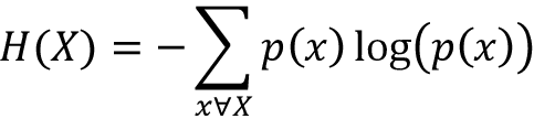
In machine learning, to optimize ML models, we measure the difference between the predicted probability distribution versus the target probability distribution for a given sample. For that, we use cross-entropy, an extension of entropy for two distributions:

Finally, we define perplexity as:

To learn more about the relationship between cross entropy and perplexity visit https://thegradient.pub/understanding-evaluation-metrics-for-language-models/.

In TensorFlow, we define a custom tf.keras.metrics.Metric object to compute perplexity. We are going to use tf.keras.metrics.Mean as our super-class as it already knows how to compute and track the mean value of a given metric:

class PerplexityMetric(tf.keras.metrics.Mean):
    def __init__(self, name='perplexity', **kwargs):
        super().__init__(name=name, **kwargs)
        self.cross_entropy = 
        tf.keras.losses.SparseCategoricalCrossentropy(
        from_logits=False, reduction='none')
    def _calculate_perplexity(self, real, pred):
        
        # The next 4 lines zero-out the padding from loss 
        # calculations, this follows the logic from: 
        # https://www.tensorflow.org/beta/tutorials/text/transformer#loss_
        # and_metrics 
        loss_ = self.cross_entropy(real, pred)
        # Calculating the perplexity steps: 
        step1 = K.mean(loss_, axis=-1)
        perplexity = K.exp(step1)
        return perplexity 
    def update_state(self, y_true, y_pred, sample_weight=None):
        perplexity = self._calculate_perplexity(y_true, y_pred)
        super().update_state(perplexity)

Here we are simply computing the cross-entropy loss for a given batch of predictions and targets using the built-in SparseCategoricalCrossentropy loss object. Then we raise it to the power of exponential to get the perplexity. We will now compile our model using:

• Sparse categorical cross-entropy as our loss function
• Adam as our optimizer
• Accuracy and perplexity as our metrics

lm_model.compile(loss='sparse_categorical_crossentropy', optimizer='adam', metrics=['accuracy', PerplexityMetric()])

Here, the perplexity metric will be tracked during model training and validation and be printed out, similar to the accuracy metric.

Training the model

It’s time to train our model. Since we have done all the heavy-lifting required (e.g. reading files, preprocessing and transforming text, and compiling the model), all we have to do is call our model with the fit() function:

lm_model.fit(train_ds, validation_data=valid_ds, epochs=60)

Here we are passing train_ds (training data pipeline) as the first argument and valid_ds (validation data pipeline) for the validation_data argument, and setting the training to run for 60 epochs. Once the model is trained, let us evaluate it on the test dataset by simply calling:

lm_model.evaluate(test_ds)

This gives the following output:

5/5 [==============================] - 0s 45ms/step - loss: 2.4742 - accuracy: 0.3968 - perplexity: 12.3155

You might have slight variations in the metrics you see, but it should roughly converge to the same value.

Defining the inference model

During training, we trained our model and evaluated it on sequences of bigrams. This works for us because during training and evaluation, we have the full text available to us. However, when we need to generate new text, we do not have anything available to us. Therefore, we have to make adjustments to our trained model so that it can generate text from scratch.

The way we do this is by defining a recursive model that takes the current time step’s output of the model as the input to the next time step. This way we can keep predicting words/bigrams for an infinite number of steps. We provide the initial seed as a random word/bigram picked from the corpus (or even a sequence of bigrams).

Figure 8.2 illustrates how the inference model works.

Figure 8.2: The operational view of the inference model we’ll be building from our trained model

Our inference model is going to be comparatively more sophisticated, as we need to design an iterative process to generate text using previous predictions as inputs. Therefore, we will be using Keras’s Functional API to implement the model:

# Define inputs to the model
inp = tf.keras.layers.Input(dtype=tf.string, shape=(1,))
inp_state_c_lstm = tf.keras.layers.Input(shape=(512,))
inp_state_h_lstm = tf.keras.layers.Input(shape=(512,))
inp_state_c_lstm_1 = tf.keras.layers.Input(shape=(256,))
inp_state_h_lstm_1 = tf.keras.layers.Input(shape=(256,))
text_vectorized_out = lm_model.get_layer('text_vectorization')(inp)
# Define embedding layer and output
emb_layer = lm_model.get_layer('embedding')
emb_out = emb_layer(text_vectorized_out)
# Defining a LSTM layers and output
lstm_layer = tf.keras.layers.LSTM(512, return_state=True, return_sequences=True)
lstm_out, lstm_state_c, lstm_state_h = lstm_layer(emb_out, initial_state=[inp_state_c_lstm, inp_state_h_lstm])
lstm_1_layer = tf.keras.layers.LSTM(256, return_state=True, return_sequences=True)
lstm_1_out, lstm_1_state_c, lstm_1_state_h = lstm_1_layer(lstm_out, initial_state=[inp_state_c_lstm_1, inp_state_h_lstm_1])
# Defining a Dense layer and output
dense_out = lm_model.get_layer('dense')(lstm_1_out)
# Defining the final Dense layer and output
final_out = lm_model.get_layer('dense_1')(dense_out)
# Copy the weights from the original model
lstm_layer.set_weights(lm_model.get_layer('lstm').get_weights())
lstm_1_layer.set_weights(lm_model.get_layer('lstm_1').get_weights())
# Define final model
infer_model = tf.keras.models.Model(
    inputs=[inp, inp_state_c_lstm, inp_state_h_lstm, 
    inp_state_c_lstm_1, inp_state_h_lstm_1], 
    outputs=[final_out, lstm_state_c, lstm_state_h, lstm_1_state_c, 
    lstm_1_state_h])

We start by defining an input layer that takes an input having one time step.

Note that we are defining the shape argument. This means it can accept an arbitrarily sized batch of data (as long as it has one time step). We also define several other inputs to maintain the states of the LSTM layers we have. This is because we have to maintain state vectors of LSTM layers explicitly as we are recursively generating outputs from the model:

inp = tf.keras.layers.Input(dtype=tf.string, shape=(1,))
inp_state_c_lstm = tf.keras.layers.Input(shape=(512,))
inp_state_h_lstm = tf.keras.layers.Input(shape=(512,))
inp_state_c_lstm_1 = tf.keras.layers.Input(shape=(256,))
inp_state_h_lstm_1 = tf.keras.layers.Input(shape=(256,))

Next we retrieve the trained model’s text_vectorization layer and transform the text to integer IDs using it:

text_vectorized_out = lm_model.get_layer('text_vectorization')(inp)

Then we obtain the embeddings layer of the train model and use it to generate the embedding output:

emb_layer = lm_model.get_layer('embedding')
emb_out = emb_layer(text_vectorized_out)

We will create a fresh new LSTM layer to represent the first LSTM layer in the trained model. This is because the inference LSTM layers will have slight differences to the trained LSTM layers. Therefore, we will define new layers and copy the trained weights over later. We set the return_state argument to True. By setting this to true we get three outputs when we call the layer with an input: the final output, the cell state, and the final state vector. Note how we are also passing another argument called initial_state. The initial_state needs to be a list of tensors: the cell state and the final state vector, in that order. We are passing the input layers as those states and will populate them accordingly during runtime:

lstm_layer = tf.keras.layers.LSTM(512, return_state=True, return_sequences=True)
lstm_out, lstm_state_c, lstm_state_h = lstm_layer(emb_out, initial_state=[inp_state_c_lstm, inp_state_h_lstm])

Similarly, the second LSTM layer will be defined. We get the dense layers and replicate the fully connected layers found in the trained model. Note that we don’t use softmax in the last layer.

This is because at inference time softmax is only an overhead, as we only need the output class with the highest output score (i.e. it doesn’t need to be a probability distribution):

# Defining a Dense layer and output
dense_out = lm_model.get_layer('dense')(lstm_1_out)
# Defining the final Dense layer and output
final_out = lm_model.get_layer('dense_1')(dense_out)

Don’t forget to copy the weights of the trained LSTM layers to our newly created LSTM layers:

lstm_layer.set_weights(lm_model.get_layer('lstm').get_weights())
lstm_1_layer.set_weights(lm_model.get_layer('lstm_1').get_weights())

Finally, we define the model:

infer_model = tf.keras.models.Model(
    inputs=[inp, inp_state_c_lstm, inp_state_h_lstm, 
    inp_state_c_lstm_1, inp_state_h_lstm_1], 
    outputs=[final_out, lstm_state_c, lstm_state_h, lstm_1_state_c, 
    lstm_1_state_h])

Our model takes a sequence of 1 bigram as the input, along with state vectors of both LSTM layers, and outputs the final prediction probabilities and the new state vectors of both LSTM layers. Let us now generate new text from the model.

Generating new text with the model

We’ll use our new inference model to generate a story. We will define an initial seed that we will use to generate a story. Here, we take the first phrase from one of the test files. Then we use it to generate text recursively, by using the predicted bigram at time t as the input at time t+1. We will run this for 500 steps:

text = ["When adam and eve were driven out of paradise, they were compelled to build a house for themselves on barren ground"]
seq = [text[0][i:i+2] for i in range(0, len(text[0]), 2)]
# build up model state using the given string
print("Making predictions from a {} element long input".format(len(seq)))
vocabulary = infer_model.get_layer("text_vectorization").get_vocabulary()
index_word = dict(zip(range(len(vocabulary)), vocabulary))
# Reset the state of the model initially
infer_model.reset_states()
# Defining the initial state as all zeros
state_c = np.zeros(shape=(1,512))
state_h = np.zeros(shape=(1,512))
state_c_1 = np.zeros(shape=(1,256))
state_h_1 = np.zeros(shape=(1,256))
# Recursively update the model by assigning new state to state
for c in seq:    
    #print(c)
    out, state_c, state_h, state_c_1, state_h_1 = infer_model.predict(
        [np.array([[c]]), state_c, state_h, state_c_1, state_h_1]
)
# Get final prediction after feeding the input string
wid = int(np.argmax(out[0],axis=-1).ravel())
word = index_word[wid]
text.append(word)
# Define first input to generate text recursively from
x = np.array([[word]])
# Code listing 10.7
for _ in range(500):
    
    # Get the next output and state
    out, state_c, state_h, state_c_1, state_h_1  = 
    infer_model.predict([x, state_c, state_h, state_c_1, state_h_1 ])
    
    # Get the word id and the word from out
    out_argsort = np.argsort(out[0], axis=-1).ravel()
    wid = int(out_argsort[-1])
    word = index_word[wid]
    
    # If the word ends with space, we introduce a bit of randomness
    # Essentially pick one of the top 3 outputs for that timestep 
    # depending on their likelihood
    if word.endswith(' '):
        if np.random.normal()>0.5:
            width = 5
            i = np.random.choice(list(range(-width,0)), 
            p=out_argsort[-width:]/out_argsort[-width:].sum())
            wid = int(out_argsort[i])    
            word = index_word[wid]
            
    # Append the prediction
    text.append(word)
    
    # Recursively make the current prediction the next input
    x = np.array([[word]])
    
# Print the final output    
print('
')
print('='*60)
print("Final text: ")
print(''.join(text))

Notice how we are recursively using the variables x, state_c, state_h, state_c_1, and state_h_1 to generate and assign new values.

    out, state_c, state_h, state_c_1, state_h_1  = 
    infer_model.predict([x, state_c, state_h, state_c_1, state_h_1 ])

Moreover, we will use a simple condition to diversify the inputs we are generating:

if word.endswith(' '):
        if np.random.normal()>0.5:
            width = 5
            i = np.random.choice(list(range(-width,0)), 
            p=out_argsort[-width:]/out_argsort[-width:].sum())
            wid = int(out_argsort[i])    
            word = index_word[wid]

Essentially, if the predicted bigram ends with the ' ' character, we will choose the next bigram randomly, from the top five bigrams. Each bigram will be chosen according to its predicted likelihood. Let’s see what the output text looks like:

When adam and eve were driven out of paradise, they were compelled to build a house for themselves on barren groundy the king's daughter and said, i will so the king's daughter angry this they were and said, "i will so the king's daughter.  the king's daughter.' they were to the forest of the stork.  then the king's daughters, and they were to the forest of the stork, and, and then they were to the forest.  ...

It seems our model is able to generate actual words and phrases that make sense. Next we will investigate how the text generated from standard LSTMs compares to other models, such as LSTMs with peepholes and GRUs.

Comparing LSTMs to LSTMs with peephole connections and GRUs

Now we will compare LSTMs to LSTMs with peepholes and GRUs in the text generation task. This will help us to compare how well different models (LSTMs with peepholes and GRUs) perform in terms of perplexity. Remember that we prefer perplexity over accuracy, as accuracy assumes there’s only one correct token given a previous input sequence. However, as we have learned, language is complex and there can be many different correct ways to generate text given previous inputs. This is available as an exercise in ch08_lstms_for_text_generation.ipynb located in the Ch08-Language-Modelling-with-LSTMs folder.

Standard LSTM

First, we will reiterate the components of a standard LSTM. We will not repeat the code for standard LSTMs as it is identical to what we discussed previously. Finally, we will see some text generated by an LSTM.

Review

Here, we will revisit what a standard LSTM looks like. As we already mentioned, an LSTM consists of the following:

• Input gate – This decides how much of the current input is written to the cell state
• Forget gate – This decides how much of the previous cell state is written to the current cell state
• Output gate – This decides how much information from the cell state is exposed to output into the external hidden state

In Figure 8.3, we illustrate how each of these gates, inputs, cell states, and the external hidden states are connected:

Figure 8.3: An LSTM cell

Gated Recurrent Units (GRUs)

Here we will first briefly delineate what a GRU is composed of, followed by showing the code for implementing a GRU cell. Finally, we look at some code generated by a GRU cell.

Review

Let’s briefly revisit what a GRU is. A GRU is an elegant simplification of the operations of an LSTM. A GRU introduces two different modifications to an LSTM (see Figure 8.4):

• It connects the internal cell state and the external hidden state into a single state
• Then it combines the input gate and the forget gate into one update gate

Figure 8.4: A GRU cell

The GRU model uses a simpler gating mechanism than the LSTM. However, it still manages to capture important capabilities such as memory updates, forgets, etc.

The model

Here we will define a GRU-based language model:

text_vectorizer = tf.keras.layers.TextVectorization(
    max_tokens=n_vocab, standardize=None,
    split=None, input_shape=(window_size,)
)
# Train the model on existing data
text_vectorizer.adapt(train_ds)
lm_gru_model = models.Sequential([
    text_vectorizer,
    layers.Embedding(n_vocab+2, 96),
    layers.GRU(512, return_sequences=True),
    layers.GRU(256, return_sequences=True),
    layers.Dense(1024, activation='relu'),
    layers.Dropout(0.5),
    layers.Dense(n_vocab, activation='softmax')
])

The training code is identical to how we trained the LSTM-based model. Therefore, we won’t duplicate our discussion here. Next we’ll look at a slightly different variant of LSTM models.

LSTMs with peepholes

Here we will discuss LSTMs with peepholes and how they are different from a standard LSTM. After that, we will discuss their implementation.

Review

Now, let’s briefly look at LSTMs with peepholes. Peepholes are essentially a way for the gates (input, forget, and output) to directly see the cell state, instead of waiting for the external hidden state (see Figure 8.5):

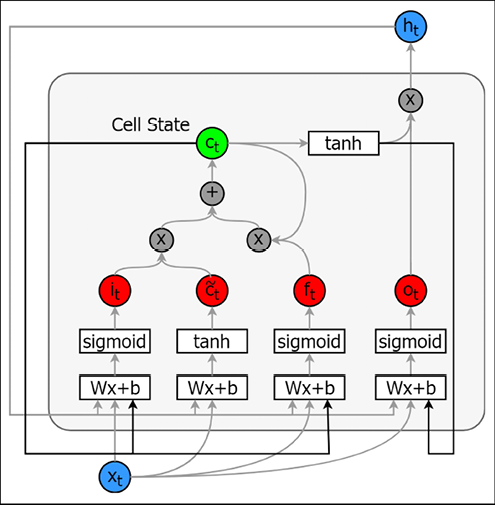
Figure 8.5: An LSTM with peepholes

The code

Note that we’re using an implementation of the peephole connections that are diagonal. We found that nondiagonal peephole connections (proposed by Gers and Schmidhuber in their paper Recurrent Nets that Time and Count, Neural Networks, 2000) hurt performance more than they help, for this language modeling task. Therefore, we’re using a different variation that uses diagonal peephole connections, as used by Sak, Senior, and Beaufays in their paper Long Short-Term Memory Recurrent Neural Network Architectures for Large Scale Acoustic Modeling, Proceedings of the Annual Conference of the International Speech Communication Association.

Fortunately, we have this technique implemented as an RNNCell object in tensorflow_addons. Therefore, all we need to do is wrap this PeepholeLSTMCell object in a layers.RNN object to produce the desired layer. The following is the code implementation:

text_vectorizer = tf.keras.layers.TextVectorization(
    max_tokens=n_vocab, standardize=None,
    split=None, input_shape=(window_size,)
)
# Train the model on existing data
text_vectorizer.adapt(train_ds)
lm_peephole_model = models.Sequential([
    text_vectorizer,
    layers.Embedding(n_vocab+2, 96),
    layers.RNN(
        tfa.rnn.PeepholeLSTMCell(512),
        return_sequences=True
    ),
    layers.RNN(
        tfa.rnn.PeepholeLSTMCell(256),
        return_sequences=True
    ),
    layers.Dense(1024, activation='relu'),
    layers.Dropout(0.5),
    layers.Dense(n_vocab, activation='softmax')
])

Now let’s look at the training and validation perplexities of different models and how they change over time.

Training and validation perplexities over time

In Figure 8.6, we have plotted the behavior of perplexity over time for LSTMs, LSTMs with peepholes, and GRUs. We can see that GRUs are a clear-cut winner in terms of performance. This can be attributed to the innovative simplification of LSTM cells found in GRU cells. But it looks like GRU model does overfit quite heavily. Therefore, it’s important to use techniques such as early stopping to prevent such behavior. We can see that LSTMs with peepholes haven’t given us much advantage in terms of performance. But it is important to keep in mind that we are using a relatively small dataset.

For larger, more complex datasets, the performance might vary. We will leave experimenting with GRU cells for the reader and continue with the LSTM model:

Figure 8.6: Perplexity change for training data over time (LSTMs, LSTM (peephole), and GRUs)

In this section, we discussed three different models: standard LSTMs, GRUs, and LSTMs with peepholes.

The results clearly indicate that, for this dataset, GRUs outperform other variants. In the next section, we will discuss techniques that can enhance the predictive power of sequential models.

Improving sequential models – beam search

As we saw earlier, the generated text can be improved. Now let’s see if beam search, which we discussed in Chapter 7, Understanding Long Short-Term Memory Networks, might help to improve the performance. The standard way to predict from a language model is by predicting one step at a time and using the prediction from the previous time step as the new input. In beam search, we predict several steps ahead before picking an input.

This enables us to pick output sequences that may not look as attractive if taken individually, but are better when considered as a sequence. The way beam search works is by, at a given time, predicting mⁿ output sequences or beams. m is known as the beam width and n is the beam depth. Each output sequence (or a beam) is n bigrams predicted into the future. We compute the joint probability of each beam by multiplying individual prediction probabilities of the items in that beam. We then pick the beam with the highest joint probability as our output sequence for that given time step. Note that this is a greedy search, meaning that we will calculate the best candidates at each depth of the tree iteratively, as the tree grows. It should be noted that this search will not result in the globally best beam. Figure 8.7 shows an example. We will indicate the best beam candidates (and their probabilities) with bold font and arrows:

Figure 8.7: A beam search illustrating the requirement for updating beam states at each step. Each number underneath the word represents the probability of that word being chosen. For the words not in bold, you can assume the probabilities are negligible

We can see that in the first step, the word “hunting” has the highest probability. However, if we perform a beam search with a beam depth of 3, we get the sequence [“king”, “was”, “hunting”] with a joint probability of 0.3 * 0.5 * 0.4 = 0.06 as the best beam.

This is higher than a beam that would start from the word “hunting” (which has a joint probability of 0.5 * 0.1 * 0.3 = 0.015).

Implementing beam search

We implement beam search as a recursive function. But first we will implement a function that performs a single step of our recursive function called beam_one_step(). This function simply takes a model, an input, and states (from the LSTM) and produces the output and new states.

def beam_one_step(model, input_, states): 
    """ Perform the model update and output for one step"""
    out = model.predict([input_, *states])
    output, new_states = out[0], out[1:]
    return output, new_states

Next, we write the main recursive function that performs beam search. This function takes the following arguments:

• model – An inference-based language model
• input_ – The initial input
• states – The initial state vectors
• beam_depth – The search depth of the beam
• beam_width – The search width of the beam (i.e. number of candidates considered at a given depth)

Let’s now discuss the function:

def beam_search(model, input_, states, beam_depth=5, beam_width=3):
    """ Defines an outer wrapper for the computational function of 
    beam search """
    vocabulary = 
    infer_model.get_layer("text_vectorization").get_vocabulary()
    index_word = dict(zip(range(len(vocabulary)), vocabulary))
    def recursive_fn(input_, states, sequence, log_prob, i):
        """ This function performs actual recursive computation of the 
        long string"""
        
        if i == beam_depth:
            """ Base case: Terminate the beam search """
            results.append((list(sequence), states, np.exp(log_prob)))
            return sequence, log_prob, states
        else:
            """ Recursive case: Keep computing the output using the 
            previous outputs"""
            output, new_states = beam_one_step(model, input_, states)
            
            # Get the top beam_width candidates for the given depth
            top_probs, top_ids = tf.nn.top_k(output, k=beam_width)
            top_probs, top_ids = top_probs.numpy().ravel(), 
            top_ids.numpy().ravel()
            # For each candidate compute the next prediction
            for p, wid in zip(top_probs, top_ids):
                new_log_prob = log_prob + np.log(p)
                
                # we are going to penalize joint probability whenever 
                # the same symbol is repeating
                if len(sequence)>0 and wid == sequence[-1]:
                    new_log_prob = new_log_prob + np.log(1e-1)
                    
                sequence.append(wid)
                _ = recursive_fn(np.array([[index_word[wid]]]), 
                new_states, sequence, new_log_prob, i+1)
                sequence.pop()
    results = []
    sequence = []
    log_prob = 0.0
    recursive_fn(input_, states, sequence, log_prob, 0)
    results = sorted(results, key=lambda x: x[2], reverse=True)
    return results

The beam_search() function in fact defines a nested recursive function (recursive_fn) that accumulates the outputs as it is called and stores the results in a list called results. The recursive_fn() does the following. If the function has been called a number of times equal to the beam_depth, then it returns the current result. If the number of function calls hasn’t reached the predefined depth, for a given depth index, then the recursive_fn():

• Computes the new output and states using the beam_one_step() function
• Gets the IDs and probabilities of the top bigram candidates
• Computes the joint probability of each beam in the log space (in log space we get better numerical stability for smaller probability values)
• Finally, we call the same function with the new inputs, new state, and the next depth index

With that you can simply call the beam_search() function to get beams of predictions from the inference model. Let’s look at how we can do that next.

Generating text with beam search

Here we will only show the part where we iteratively call beam_search() to generate new text. For the full code refer to ch08_lstms_for_text_generation.ipynb.

for i in range(50):
    print('.', end='')
    # Get the results from beam search
    result = beam_search(infer_model, x, states, 5, 5)
    
    # Get one of the top 10 results based on their likelihood
    n_probs = np.array([p for _,_,p in result[:10]])
    p_j = np.random.choice(list(range(n_probs.size)), 
    p=n_probs/n_probs.sum())                    
    best_beam_ids, states, _ = result[p_j]
    x = np.array([[index_word[best_beam_ids[-1]]]])
    text.extend([index_word[w] for w in best_beam_ids])

We simply call the function beam_search() with infer_model, current input x, current states states, beam depth, and beam width, and update x and states to reflect the winning beam. Then the model will iteratively use the winning beam to produce the next beam.

Let’s see how our LSTM performs with beam search:

When adam and eve were driven out of paradise, they were compelled to build a house for themselves on barren groundr, said the king's daughter went out of the king's son to the king's daughter, and then the king's daughter went into the world, and asked the hedgehog's daughter that the king was about to the forest, and there was on the window, and said, "if you will give her that you have been and said, i will give him the king's daughter, but when she went to the king's sister, and when she was still before the window, and said to himself, and when he said to her father, and that he had nothing and said to hi

Here’s what the standard LSTM with greedy sampling (i.e. predicting one word at a time) outputs:

When adam and eve were driven out of paradise, they were compelled to build a house for themselves on barren groundr, and then this they were all the third began to be able to the forests, and they were.  the king's daughter was no one was about to the king's daughter to the forest of them to the stone.  then the king's daughter was, and then the king's daughter was nothing-eyes, and the king's daughter was still, and then that had there was about through the third, and the king's daughters was seems to the king's daughter to the forest of them to the stone for them to the forests, and that it was not been to be ables, and the king's daughter wanted to be and said, ...

Compared to the text produced by the LSTM, this text seems to have more variation in it while keeping the text grammatically consistent as well. So, in fact, beam search helps to produce quality predictions compared to predicting one word at a time. But still, there are instances where words together don’t make much sense. Let’s see how we can improve our LSTM further.

Improving LSTMs – generating text with words instead of n-grams

Here we will discuss ways to improve LSTMs. We have so far used bigrams as our basic unit of text. But you would get better results by incorporating words, as opposed to bigrams. This is because using words reduces the overhead of the model by alleviating the need to learn to form words from bigrams. We will discuss how we can employ word vectors in the code to generate better-quality text compared to using bigrams.

The curse of dimensionality

One major limitation stopping us from using words instead of n-grams as the input to our LSTM is that this will drastically increase the number of parameters in our model. Let’s understand this through an example. Consider that we have an input of size 500 and a cell state of size 100. This would result in a total of approximately 240K parameters (excluding the softmax layer), as shown here:

Let’s now increase the size of the input to 1000. Now the total number of parameters would be approximately 440K, as shown here:

As you can see, for an increase of 500 units of the input dimensionality, the number of parameters has grown by 200,000. This not only increases the computational complexity but also increases the risk of overfitting due to the large number of parameters. So, we need ways of restricting the dimensionality of the input.

Word2vec to the rescue

As you will remember, not only can Word2vec give a lower-dimensional feature representation of words compared to one-hot encoding, but it also gives semantically sound features. To understand this, let’s consider three words: cat, dog, and volcano. If we one-hot encode just these words and calculate the Euclidean distance between them, it would be the following:

distance(cat,volcano) = distance(cat,dog)

However, if we learn word embeddings, it would be the following:

distance(cat,volcano) > distance(cat,dog)

We would like our features to represent the latter, where similar things have a lower distance than dissimilar things. Consequently, the model will be able to generate better-quality text.

Generating text with Word2vec

The structure of the model remains more or less the same as what we have discussed. It is only the units of text we would consider that changes.

Figure 8.8 depicts the overall architecture of LSTM-Word2vec:

Figure 8.8: The structure of a language modeling LSTM using word vectors

You have a few options when it comes to using word vectors. You can either:

• Randomly initialize the vectors and jointly learn them during the task
• Train the embeddings using a word vector algorithm (e.g. Word2vec, GloVe, etc.) beforehand
• Use pretrained word vectors freely available to download, to initialize the embedding layer

We end our discussion on language modeling here.

Summary

In this chapter, we looked at the implementations of the LSTM algorithm and other various important aspects to improve LSTMs beyond standard performance. As an exercise, we trained our LSTM on the text of stories by the Grimm brothers and asked the LSTM to output a fresh new story. We discussed how to implement an LSTM model with code examples extracted from exercises.

Next, we had a technical discussion about how to implement LSTMs with peepholes and GRUs. Then we did a performance comparison between a standard LSTM and its variants. We saw that the GRUs performed the best compared to LSTMs with peepholes and LSTMs.

Then we discussed some of the various improvements possible for enhancing the quality of outputs generated by an LSTM. The first improvement was beam search. We looked at an implementation of beam search and covered how to implement it step by step. Then we looked at how we can use word embeddings to teach our LSTM to output better text.

In conclusion, LSTMs are very powerful machine learning models that can capture both long-term and short-term dependencies.

Moreover, beam search in fact helps to produce more realistic-looking textual phrases compared to predicting one at a time.

In the next chapter, we will look at how sequential models can be used to solve a more complex type of problem known as sequence-to-sequence problems. Specifically, we will look at how we can perform machine translation by formulating it as a sequence-to-sequence problem.

To access the code files for this book, visit our GitHub page at: https://packt.link/nlpgithub

Join our Discord community to meet like-minded people and learn alongside more than 1000 members at: https://packt.link/nlp