11

Image Captioning with Transformers

Transformer models changed the playing field for many NLP problems. They have redefined the state of the art by a significant margin, compared to the previous leaders: RNN-based models. We have already studied Transformers and understood what makes them tick. Transformers have access to the whole sequence of items (e.g. a sequence of tokens), as opposed to RNN-based models that look at one item at a time, making them well-suited for sequential problems. Following their success in the field of NLP, researchers have successfully used Transformers to solve computer vision problems. Here we will learn how to use Transformers to solve a multi-modal problem involving both images and text: image captioning.

Automated image captioning, or image annotation, has a wide variety of applications. One of the most prominent applications is image retrieval in search engines. Automated image captioning can be used to retrieve all the images belonging to a certain class (for example, a cat) as per the user’s request. Another application can be in social media where, when an image is uploaded by a user, the image is automatically captioned so that the user can either refine the generated caption or post it as it is.

In this chapter, we will learn to caption images using machine learning, where a model is trained to generate a sequence of tokens (i.e. a caption) when given an image. We will first understand how Transformer models are used in computer vision, and then extend our understanding to solve the problem of generating captions for images. For generating captions for images, we will use a popular dataset for image captioning tasks known as Microsoft Common Objects in Context (MS-COCO).

Solving this will require two Transformer models: one to generate an image representation and the other to generate the relevant caption. Once the image representation is generated, it will be fed as one of the inputs to the text-based Transformer model. The text-based Transformer model will be trained to predict the next token in the caption given the current caption, at a given time step.

We will generate three datasets: training, validation, and testing datasets. We use the training dataset to train the model and the validation set to monitor performance during training. Finally we use the test dataset to generate captions for a set of unseen images.

Looking at the image caption generation pipeline at a very high level, we have two main components:

1. A pretrained Vision Transformer model that takes in an image and produces a 1D hidden representation of the image
2. A text-based Transformer decoder model that can decode the hidden image representation to a series of token IDs

We will use a pretrained Transformer model to generate image representations. Known as the Vision Transformer (ViT), it has been trained on the ImageNet dataset and has delivered great performance on the ImageNet classification task.

Specifically, this chapter will cover the following main topics:

• Getting to know the data
• Downloading the data
• Processing and tokenizing data
• Defining a tf.data.Dataset
• The machine learning pipeline for image caption generation
• Implementing the model with TensorFlow
• Training the model
• Evaluating the results quantitatively
• Evaluating the model
• Captions generated for test images

Getting to know the data

Let’s first understand the data we are working with both directly and indirectly. There are two datasets we will rely on:

• The ILSVRC ImageNet dataset (http://image-net.org/download)
• The MS-COCO dataset (http://cocodataset.org/#download)

We will not engage the first dataset directly, but it is essential for caption learning. This dataset contains images and their respective class labels (for example, cat, dog, and car). We will use a CNN that is already trained on this dataset, so we do not have to download and train on this dataset from scratch. Next we will use the MS-COCO dataset, which contains images and their respective captions. We will directly learn from this dataset by mapping the image to a fixed-size feature vector, using the Vision Transformer, and then map this vector to the corresponding caption using a text-based Transformer (we will discuss this process in detail later).

ILSVRC ImageNet dataset

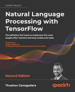
ImageNet is an image dataset that contains a large set of images (~1 million) and their respective labels. These images belong to 1,000 different categories. This dataset is very expressive and contains almost all the objects found in the images we want to generate captions for. Figure 11.1 shows some of the classes available in the ImageNet dataset:

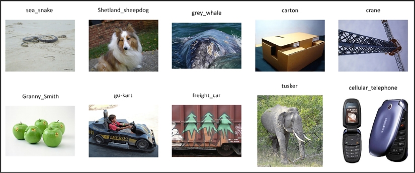
Figure 11.1: A small sample of the ImageNet dataset

ImageNet is a good dataset to train on, in order to obtain image encodings that are required for caption generation. We say we use this dataset indirectly because we will use a pretrained Transformer that is trained on this dataset. Therefore, we will not be downloading, nor training the model on this dataset, by ourselves.

The MS-COCO dataset

Now we will move on to the dataset that we will actually be using, which is called MS-COCO (short for Microsoft - Common Objects in Context). We will use the training dataset from the year 2014 and the validation set from 2017. We use datasets belonging to different times to avoid using large datasets for this exercise. As described earlier, this dataset consists of images and their respective descriptions. The dataset is quite large (for example, the training dataset consists of ~120,000 samples and can measure over 15 GB). Datasets are updated every year, and a competition is then held to recognize the team that achieves state-of-the-art performance. Using the full dataset is important when the objective is to achieve state-of-the-art performance. However, in our case, we want to learn a reasonable model that is able to suggest what is in an image generally. Therefore, we will use a smaller dataset (~40,000 images and ~200,000 captions) to train our model. Figure 11.2 includes some of the samples available:

Figure 11.2: A small sample of the MS-COCO dataset

For learning with and testing our end-to-end image caption generation model, we will use the 2017 validation dataset, provided on the official MS-COCO dataset website.

In Figure 11.3, we can see some of the images found in the validation set. These are some hand-picked examples from the validation set representing a variety of different objects and scenes:

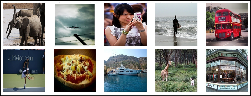
Figure 11.3: Unseen images that we will use to test the image caption generation capability of our algorithm

Downloading the data

The MS-COCO dataset we will be using is quite large. Therefore, we will manually download these datasets. To do that, follow the instructions below:

1. Create a folder called data in the Ch11-Image-Caption-Generation folder
2. Download the 2014 Train images set (http://images.cocodataset.org/zips/train2014.zip) containing 83K images (train2014.zip)
3. Download the 2017 Val images set (http://images.cocodataset.org/zips/val2017.zip) containing 5K images (val2017.zip)
4. Download the annotation sets for 2014 (annotations_trainval2014.zip) (http://images.cocodataset.org/annotations/annotations_trainval2014.zip) and 2017 (annotations_trainval2017.zip) (http://images.cocodataset.org/annotations/annotations_trainval2017.zip)
5. Copy the downloaded zip files to the Ch11-Image-Caption-Generation/data folder
6. Extract the zip files using the Extract to option so that it unzips the content within a sub-folder

Once you complete the above steps, you should have the following subfolders:

• data/train2014 – Contains the training images
• data/annotations_trainval2014 – Contains the captions of the training images
• data/val2017 – Contains the validation images
• data/annotations_trainval2017 – Contains the captions of the validation images

Processing and tokenizing data

With the data downloaded and placed in the correct folders, let’s define the directories containing the required data:

trainval_image_dir = os.path.join('data', 'train2014', 'train2014')
trainval_captions_dir = os.path.join('data', 'annotations_trainval2014', 'annotations')
test_image_dir = os.path.join('data', 'val2017', 'val2017')
test_captions_dir = os.path.join('data', 'annotations_trainval2017', 'annotations')
trainval_captions_filepath = os.path.join(trainval_captions_dir, 'captions_train2014.json')
test_captions_filepath = os.path.join(test_captions_dir, 'captions_val2017.json')

Here we have defined the directories containing training and testing images as well as the file paths of the JSON files that contain the captions of the training and testing images.

Preprocessing data

As the next step, let’s split the training set in to train and validation sets. We will use 80% of the original set as training data and 20% as the validation data (randomly chosen):

all_filepaths = np.array([os.path.join(trainval_image_dir, f) for f in os.listdir(trainval_image_dir)])
rand_indices = np.arange(len(all_filepaths))
np.random.shuffle(rand_indices)
split = int(len(all_filepaths)*0.8)
train_filepaths, valid_filepaths = all_filepaths[rand_indices[:split]], all_filepaths[rand_indices[split:]] 

We can print the dataset sizes and see what we ended up with:

print(f"Train dataset size: {len(train_filepaths)}")
print(f"Valid dataset size: {len(valid_filepaths)}")

This will print:

Train dataset size: 66226
Valid dataset size: 16557

Now let’s read the captions and create a pandas DataFrame using them. Our DataFrame will have four important columns:

• image_id – Identifies an image (used to generate the file path)
• image_filepath – File location of the image identified by image_id
• caption – Original caption
• preprocessed_caption – Caption after some simple preprocessing

First we will load the data in the JSON file and get the data into a DataFrame:

with open(trainval_captions_filepath, 'r') as f:
    trainval_data = json.load(f)
trainval_captions_df = pd.json_normalize(trainval_data, "annotations")

The data we’re looking for in the file is found under a key called "annotations". Under "annotations" we have a list of dictionaries each having the image_id, id, and caption. The function pd.json_normalize() takes in the loaded data and converts that to a pd.DataFrame.

We then create the column called image_filepath by prefixing the root directory path to the image_id and appending the extension .jpg.

We will only keep the data points where the image_filepath values are in the training images we stored in train_filepaths:

trainval_captions_df["image_filepath"] = trainval_captions_df["image_id"].apply(
    lambda x: os.path.join(trainval_image_dir, 
    'COCO_train2014_'+format(x, '012d')+'.jpg')
)
train_captions_df = trainval_captions_df[trainval_captions_df["image_filepath"].isin(train_filepaths)]

We now define a function called preprocess_captions() that processes the original caption:

def preprocess_captions(image_captions_df):
    """ Preprocessing the captions """
    
    image_captions_df["preprocessed_caption"] = "[START] " + 
    image_captions_df["caption"].str.lower().str.replace('[^ws]','') 
    + " [END]"
    return image_captions_df

In the above code, we:

• Added two special tokens, [START] and [END], to denote the start and the end of each caption respectively
• Converted the captions to lowercase
• Removed everything that is not a word, character, or space

We then call this function on the training dataset:

train_captions_df = preprocess_captions(train_captions_df)

We then follow a similar process for both validation and test data:

valid_captions_df = trainval_captions_df[
    trainval_captions_df[
        "image_filepath"
    ].isin(valid_filepaths)
]
valid_captions_df = preprocess_captions(valid_captions_df)
with open(test_captions_filepath, 'r') as f:
    test_data = json.load(f)
    
test_captions_df = pd.json_normalize(test_data, "annotations")
test_captions_df["image_filepath"] = test_captions_df["image_id"].apply(
    lambda x: os.path.join(test_image_dir, format(x, '012d')+'.jpg')
)
test_captions_df = preprocess_captions(test_captions_df)

Let’s check the data in training_captions_df (Figure 11.4):

Figure 11.4: Data contained in training_captions_df

This data shows important information such as where the image is located in the file structure, the original caption, and the preprocessed caption.

Let’s also analyze some statistics about the images. We will take a small sample of the first 1,000 images from the training dataset and look at image sizes:

n_samples = 1000
train_image_stats_df = train_captions_df.loc[:n_samples, "image_filepath"].apply(lambda x: Image.open(x).size)
train_image_stats_df = pd.DataFrame(train_image_stats_df.tolist(), index=train_image_stats_df.index)
train_image_stats_df.describe()

This will produce Figure 11.5:

Figure 11.5: Statistics about the size of the images in the training dataset

We can see that most images have a resolution of 640x640. We will later need to resize images to 224x224 to match the model’s input requirements. We’ll also look at our vocabulary size:

train_vocabulary = train_captions_df["preprocessed_caption"].str.split(" ").explode().value_counts()
print(len(train_vocabulary[train_vocabulary>=25]))

This prints:

3629

This tells us that 3,629 words occur at least 25 times in our train dataset. We use this as our vocabulary size.

Tokenizing data

Since we are developing Transformer models, we need a robust tokenizer similar to the ones used by popular models like BERT. Hugging Face’s tokenizers library provides us with a range of tokenizers that are easy to use. Let’s understand how we can use one of these tokenizers for our purpose. You can import it using:

from tokenizers import BertWordPieceTokenizer

Next, let’s define the BertWordPieceTokenizer. We will pass the following arguments when doing so:

• unk_token – Defines a token to be used for out-of-vocabulary words
• clean_text – Whether to perform simple preprocessing steps to clean text
• lowercase – Whether to lowercase the text

These arguments can be seen in the following:

# Initialize an empty BERT tokenizer
tokenizer = BertWordPieceTokenizer(
    unk_token="[UNK]",
    clean_text=False,
    lowercase=False,
)

With the tokenizer defined, we can call the train_from_iterator() function to train the tokenizer on our dataset:

tokenizer.train_from_iterator(

    train_captions_df["preprocessed_caption"].tolist(),
    vocab_size=4000,
    special_tokens=["[PAD]", "[UNK]", "[START]", "[END]"]
)

The train_from_iterator() function takes in several arguments:

• iterator – An iterable that produces a string (containing the caption) as one item.
• vocab_size – Size of the vocabulary.
• special_tokens – Special tokens that will be used in our data. Specifically we use [PAD] (to denote padding), [UNK] (to denote OOV tokens), [START] (to denote the start), and [END] (to denote the end). These tokens will get assigned lower IDs starting from 0.

Once the tokenizer is trained, we can use it to convert strings of text to sequences of tokens. Let’s convert a few example sentences to sequences of tokens using the trained tokenizer:

# Encoding a sentence
example_captions = valid_captions_df["preprocessed_caption"].iloc[:10].tolist()
example_tokenized_captions = tokenizer.encode_batch(example_captions)
for caption, tokenized_cap in zip(example_captions, example_tokenized_captions):
    print(f"{caption} -> {tokenized_cap.tokens}") 

This will print:

[START] an empty kitchen with white and black appliances [END] -> ['[START]', 'an', 'empty', 'kitchen', 'with', 'white', 'and', 'black', 'appliances', '[END]']
[START] a white square kitchen with tile floor that needs repairs  [END] -> ['[START]', 'a', 'white', 'square', 'kitchen', 'with', 'tile', 'floor', 'that', 'need', '##s', 'rep', '##air', '##s', '[END]']
[START] a few people sit on a dim transportation system  [END] -> ['[START]', 'a', 'few', 'people', 'sit', 'on', 'a', 'dim', 'transport', '##ation', 'system', '[END]']
[START] a person protected from the rain by their umbrella walks down the road [END] -> ['[START]', 'a', 'person', 'prote', '##cted', 'from', 
'the', 'rain', 'by', 'their', 'umbrella', 'walks', 'down', 'the', 'road', '[END]']
[START] a white kitchen in a home with the light on [END] -> ['[START]', 'a', 'white', 'kitchen', 'in', 'a', 'home', 'with', 'the', 'light', 'on', '[END]']

You can see how the tokenizer has learned its own vocabulary and is tokenizing string sentences. The words that contain ## in front mean they must be combined with the previous token (without spaces) to get the final result. For example, the final string from the tokens 'image', 'cap' and '##tion' is 'image caption'. Let’s see which IDs the special tokens we defined are mapped to:

vocab = tokenizer.get_vocab()
for token in ["[UNK]", "[PAD]", "[START]", "[END]"]:
    print(f"{token} -> {vocab[token]}")

This will output:

[UNK] -> 1
[PAD] -> 0
[START] -> 2
[END] -> 3

Now let’s look at how we can define a TensorFlow data pipeline using the processed data.

Defining a tf.data.Dataset

Now let’s look at how we can create a tf.data.Dataset using the data. We will first write a few helper functions. Namely, we’ll define:

• parse_image() to load and process an image from a filepath
• generate_tokenizer() to generate a tokenizer trained on the data passed to the function

First let’s discuss the parse_image() function. It takes three arguments:

• filepath – Location of the image
• resize_height – Height to resize the image to
• resize_width – Width to resize the image to

The function is defined as follows:

def parse_image(filepath, resize_height, resize_width):
    """ Reading an image from a given filepath """
    
    # Reading the image
    image = tf.io.read_file(filepath)
    # Decode the JPEG, make sure there are 3 channels in the output
    image = tf.io.decode_jpeg(image, channels=3)
    image = tf.image.convert_image_dtype(image, tf.float32)
    # Resize the image to 224x224
    image = tf.image.resize(image, [resize_height, resize_width])
    
    # Bring pixel values to [-1, 1]
    image = image*2.0 - 1.0
        
    return image

We are mostly relying on tf.image functions to load and process the image. This function specifically:

• Reads the image from the filepath
• Decodes the bytes in the JPEG image to a uint8 tensor and converts to a float32 dtype tensor.

By the end of these steps, we’ll have an image whose pixel values are between 0 and 1. Next, we:

• Resize the image to a given height and width
• Finally normalize the image so that the pixel values are between -1 and 1 (as required by the ViT model we’ll be using)

With that we define the second helper function. This function encapsulates the functionality of the BertWordPieceTokenizer we have discussed previously:

def generate_tokenizer(captions_df, n_vocab):
    """ Generate the tokenizer with given captions """
    
    # Define the tokenizer
    tokenizer = BertWordPieceTokenizer(
        unk_token="[UNK]",
        clean_text=False,
        lowercase=False,
    )
    
    # Train the tokenizer
    tokenizer.train_from_iterator(
        captions_df["preprocessed_caption"].tolist(),
        vocab_size=n_vocab,
        special_tokens=["[PAD]", "[UNK]", "[START]", "[END]"]
    )
    
    return tokenizer

With that we can define our main data function to generate the TensorFlow data pipeline:

def generate_tf_dataset(
    image_captions_df, tokenizer=None, n_vocab=5000, pad_length=33, batch_size=32, training=False
):
    """ Generate the tf.data.Dataset"""
    
    # If the tokenizer is not available, create one
    if not tokenizer:
        tokenizer = generate_tokenizer(image_captions_df, n_vocab)
        
    # Get the caption IDs using the tokenizer
    image_captions_df["caption_token_ids"] = [enc.ids for enc in 
    tokenizer.encode_batch(image_captions_df["preprocessed_caption"])]
    
    vocab = tokenizer.get_vocab()
    
    # Add the padding to short sentences and truncate long ones
    image_captions_df["caption_token_ids"] = 
    image_captions_df["caption_token_ids"].apply(
        lambda x: x+[vocab["[PAD]"]]*(pad_length - len(x) + 2) if 
        pad_length + 2 >= len(x) else x[:pad_length + 1] + [x[-1]]
    ) 
    
    # Create a dataset with images and captions
    dataset = tf.data.Dataset.from_tensor_slices({
        "image_filepath": image_captions_df["image_filepath"],
        "caption_token_ids": 
        np.array(image_captions_df["caption_token_ids"].tolist())
    })
    
    # Each sample in our dataset consists of (image, caption token 
    # IDs, position IDs), (caption token IDs offset by 1)
    dataset = dataset.map(
        lambda x: (
            (parse_image(x["image_filepath"], 224, 224), 
            x["caption_token_ids"][:-1], tf.range(pad_length+1, 
            dtype='float32')), x["caption_token_ids"]
        )
    )
    
    # Shuffle and batch data in the training mode
    if training:
        dataset = dataset.shuffle(buffer_size=batch_size*10)
    
    dataset = dataset.batch(batch_size)
    
    return dataset, tokenizer

This function takes the following arguments:

• image_captions_df – A pandas DataFrame containing image file paths and processed captions
• tokenizer – An optional tokenizer that will be used to tokenize the captions
• n_vocab – The vocabulary size
• pad_length – The length to pad captions
• batch_size – Batch size to batch the data
• training – Whether the data pipeline should be run in training mode or not. In training mode, we shuffle data whereas otherwise, we do not

First this function generates a tokenizer if a new tokenizer has not been passed. Next we create a column called “caption_token_ids" in our DataFrame, which is created by calling the encode_batch() function of the tokenizer on the preprocessed_caption column. We then perform padding on the caption_token_ids column. We add the [PAD] token ID if a caption is shorter than pad_length, or truncate it if it’s longer. We then create a tf.data.Dataset using the from_tensor_slices() function.

Each sample in this dataset will be a dictionary with the key image_filepath and caption_token_ids and values containing corresponding values. Once we do this, we have the ingredients to get the actual data. We will call the tf.data.Dataset.map() function to:

• Call parse_image() on each image_filepath to produce the actual image
• Return all caption token IDs, except the last, as inputs
• A range from 0 to the number of tokens, representing position of each input token ID (used to get positional embeddings for the Transformer)
• Return all caption token IDs as the targets

Let’s understand what the inputs and outputs are going to look like for an example. Say you have the caption a brown bear. Here’s how the inputs and outputs going to look for our Transformer decoder (Figure 11.6):

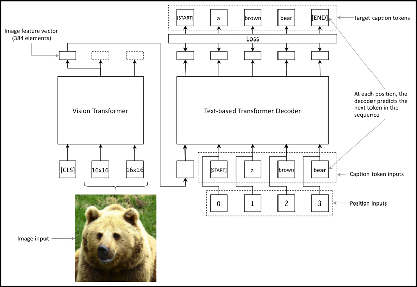
Figure 11.6: How inputs and targets are organized for the model

Finally, if in training mode, we shuffle the dataset using a buffer_size of 10 times the batch size. Then we batch the dataset using the batch_size provided when calling the function. Let’s call this function on our training dataset to see what we get:

n_vocab=4000
batch_size=2
sample_dataset, sample_tokenizer = generate_tf_dataset(train_captions_df, n_vocab=n_vocab, pad_length=10, batch_size=batch_size, training=True)
for i in sample_dataset.take(1):
    print(i)

Which will output:

(
    (
        <tf.Tensor: shape=(2, 224, 224, 3), dtype=float32, numpy=
         array([[[[-0.2051357 , -0.22082198, -0.31493968],
         [-0.2015593 , -0.21724558, -0.31136328],
         [-0.17017174, -0.18585801, -0.2799757 ],
         ...,
         [-0.29620153, -0.437378  , -0.6155298 ],
         [-0.28843057, -0.41392076, -0.6178423 ],
         [-0.29654706, -0.43772352, -0.62483776]],
        [[-0.8097613 , -0.6725868 , -0.55734015],
         [-0.7580646 , -0.6420185 , -0.55782473],
         [-0.77606916, -0.67418844, -0.5419755 ],
         ...,
         [-0.6400192 , -0.4753132 , -0.24786222],
         [-0.70908225, -0.5426947 , -0.31580424],
         [-0.7206869 , -0.5324516 , -0.3128438 ]]]], dtype=float32)>,
 
        <tf.Tensor: shape=(2, 11), dtype=int32, numpy=
         array([[   2,   24,  356,  114,  488, 1171, 1037, 2820,  566,  445,  116],
         [   2,   24, 1357, 2142,   63, 1473,  495,  282,  116,   24,  301]])>, 
        <tf.Tensor: shape=(2, 11), dtype=float32, numpy=
         array([[ 0.,  1.,  2.,  3.,  4.,  5.,  6.,  7.,  8.,  9., 10.],
         [ 0.,  1.,  2.,  3.,  4.,  5.,  6.,  7.,  8.,  9., 10.]],
      dtype=float32)>
    ), 
    <tf.Tensor: shape=(2, 12), dtype=int32, numpy=
     array([[   2,   24,  356,  114,  488, 1171, 1037, 2820,  566,  445,  116,
           3],
     [   2,   24, 1357, 2142,   63, 1473,  495,  282,  116,   24,  301,
           3]])>
)

Here we can see the inputs and outputs organized into a nested tuple. It has the format ((image, input caption token IDs, position IDs), target caption token IDs). For example, we have produced a data pipeline with a batch size of 2, a pad length of 10, and a vocabulary size of 4,000. We can see the image batch has the shape [2, 224, 224, 3], input caption token IDs and the position IDs have the shape [2, 11], and finally, the target caption token IDs are of shape [2, 12]. It is important to note that we use an additional buffer for padding length to incorporate the [START] and [END] tags. Therefore, the resulting tensors use a caption length of 12 (i.e. 10+2). The most important thing to note here is the length of the input and target captions. Input captions have one item less than the target captions as shown by the lengths. This is because, the first item in our input captions would be the image feature vector. This brings the length of input tokens to be equal to the length of target tokens.

With the data pipeline out of the way, we will discuss the mechanics of the model we’ll be using.

The machine learning pipeline for image caption generation

Here we will look at the image caption generation pipeline at a very high level and then discuss it piece by piece until we have the full model. The image caption generation framework consists of two main components:

• A pretrained Vision Transformer model to produce an image representation
• A text-based decoder model that can decode the image representation to a series of token IDs. This uses a text tokenizer to convert tokens to token IDs and vice versa

Though the Transformer models were initially used for text-based NLP problems, they have out-grown the domain of text data and have been used in other areas such as image data and audio data.

Here we will be using one Transformer model that can process image data and another that can process text data.

Vision Transformer (ViT)

First, let’s look at the Transformer generating the encoded vector representations of images. We will be using a pretrained Vision Transformer (ViT) to achieve this. This model has been trained on the ImageNet dataset we discussed above. Let’s understand the architecture of this model.

Originally, the ViT was proposed in the paper An Image is Worth 16X16 Words: Transformers for Image Recognition at Scale by Dosovitskiy et al (https://arxiv.org/pdf/2010.11929.pdf). This can be considered the first substantial step toward adapting Transformers for computer vision problems. This model is called the Vision Transformer model.

The idea is to decompose an image into small patches of 16x16 and consider each as a separate token. Each image path is flattened to a 1D vector and their position is encoded by a positional encoding mechanism similar to the original Transformer. But images are 2D structures; is it enough to have 1D positional information, and not 2D positional information? The authors argue that a 1D positional encoding was adequate and 2D positional encoding did not provide a significant boost. Once the image is broken into patches of 16x16 and flattened, each image can be presented as a sequence of tokens, just like a textual input sequence (Figure 11.7).

Then the model is pretrained in a self-supervised fashion, using a vision dataset called JFT-300M (https://paperswithcode.com/dataset/jft-300m). The paper proposes an elegant way to train the ViT in a semi-supervised fashion using image data. Similar to how NLP problems represent a unit of text as a token, a token is a patch of an image (i.e. a sequence of continuous values where values are normalized pixels). Then the ViT is pretrained to predict the mean 3-bit RGB color of a given image patch. Each channel (i.e. red, green, and blue) is represented with 3 bits (each bit having a value of 0 or 1), which gives 512 possibilities or classes. In other words, for a given image, patches (similar to how tokens are treated in NLP) are masked randomly (using the same approach as BERT), and the model is asked to predict the mean 3-bit RGB color of that image patch.

After pretraining, the model can be fine-tuned for a task-specific problem by fitting a classification or a regression head on top of the ViT, just like BERT. The ViT also has the [CLS] token at the beginning of the sequence, which will be used as the input representation for downstream vision models that are plugged on top of the ViT.

Figure 11.7 illustrates the mechanics of the ViT:

Figure 11.7: The Vision Transformer model

The model we’ll be using here originated from the paper How to train your ViT? Data, Augmentation, and Regularization in Vision Transformers by Steiner et al (https://arxiv.org/pdf/2106.10270.pdf). It proposes several variants of the ViT model. Specifically, we will use the ViT-S/16 architecture. ViT-S is the second smallest ViT model with 12 layers and a hidden output dimensionality of 384; in total it has 22.2M parameters. The number 16 here means that the model is trained on image patches of 16x16. The model has been fine-tuned using the ImageNet dataset we discussed earlier. We will use the feature extractor part of the model for the purpose of image captioning.

Text-based decoder Transformer

The text-based decoder’s primary purpose is to predict the next token in the sequence given the previous tokens. This decoder is mostly similar to the BERT we used in the previous chapter. Let’s refresh our memory on what the Transformer model is composed of. The Transformer consists of several stacked layers. Each layer has:

• A self-attention layer – Generates a hidden representation for each token position by taking in the input token and attending to the tokens at other positions in the sequence
• A fully connected subnetwork – Generates an element-wise non-linear hidden representation by propagating the self-attention layer’s output through two fully connected layers

In addition to these, the network uses residual connections and layer normalization techniques to enhance performance. When speaking of inputs, the model uses two types of input embeddings to inform the model:

• Token embeddings – Each token is represented with an embedding vector that is jointly trained with the model
• Position embeddings – Each token position is represented by an ID and a corresponding embedding for that position

Compared to the BERT we used in the previous chapter, a key difference in our model is how we use the self-attention mechanism. When using BERT, the self-attention layer was able to pay attention in a bidirectional manner (i.e. pay attention to tokens on both sides of the current input). However, in the decoder-based model, it can only pay attention to the tokens to the left of the current token. In other words, the attention mechanism only has access to inputs seen up to the current input.

Putting everything together

Let’s now learn how to put the two models together. We will use the following procedure to train the model end to end:

1. We generate the image encoding via the ViT model. It generates a single representation of 384 items for an image.
2. This representation, along with all the caption tokens except the last, goes into the decoder as the inputs.
3. Given the current input token, the decoder predicts the next token. At the end of this process we will have the full image caption.

Another alternative for connecting the ViT and the text decoder models is by providing direct access to the ViT’s full sequence of encoder outputs as a part of the attention mechanism of the decoder. In this work, not to overcomplicate our discussion, we only use a single output from the ViT model as an input to the decoder.

Implementing the model with TensorFlow

We will now implement the model we just studied. First let’s import a few things:

import tensorflow_hub as hub
import tensorflow as tf
import tensorflow.keras.backend as K

Implementing the ViT model

Next, we are going to download the pretrained ViT model from TensorFlow Hub. We will be using a model submitted by Sayak Paul. The model is available at https://tfhub.dev/sayakpaul/vit_s16_fe/1. You can see other Vision Transformer models available at https://tfhub.dev/sayakpaul/collections/vision_transformer/1.

image_encoder = hub.KerasLayer("https://tfhub.dev/sayakpaul/vit_s16_fe/1", trainable=False)

We then define an input layer to input images and pass that to the image_encoder to get the final feature vector for that image:

image_input = tf.keras.layers.Input(shape=(224, 224, 3))
image_features = image_encoder(image_input)

You can look at the size of the final image representation by running:

print(f"Final representation shape: {image_features.shape}")

which will output:

Final representation shape: (None, 384)

Next we will look at the details of how to implement the text-based Transformer model, which will take in the image representation to generate the image caption.

Implementing the text-based decoder

Here we will implement a Transformer decoder model from the ground up. This is different from how we used Transformer models before, where we downloaded a pretrained model and used them.

Before we implement the model itself, we are going to implement two custom Keras layers: one for the self-attention mechanism and the other one to capture the functionality of a single layer in the Transformer model. Let’s start with the self-attention layer.

Defining the self-attention layer

Here we define the self-attention layer using the Keras subclassing API:

class SelfAttentionLayer(tf.keras.layers.Layer):
    """ Defines the computations in the self attention layer """
    
    def __init__(self, d):        
        super(SelfAttentionLayer, self).__init__()
        # Feature dimensionality of the output
        self.d = d
    
    def build(self, input_shape):
        # Query weight matrix
        self.Wq = self.add_weight(
            shape=(input_shape[-1], self.d), 
            initializer='glorot_uniform',
            trainable=True, dtype='float32'
        )        
        # Key weight matrix
        self.Wk = self.add_weight(
            shape=(input_shape[-1], self.d), 
            initializer='glorot_uniform',
            trainable=True, dtype='float32'
        )
        # Value weight matrix
        self.Wv = self.add_weight(
            shape=(input_shape[-1], self.d), 
            initializer='glorot_uniform',
            trainable=True, dtype='float32'
        )
    
    def call(self, q_x, k_x, v_x, mask=None):
        
        q = tf.matmul(q_x,self.Wq) #[None, t, d]
        k = tf.matmul(k_x,self.Wk) #[None, t, d]
        v = tf.matmul(v_x,self.Wv) #[None, t, d]
        
        # Computing the final output
        h = tf.keras.layers.Attention(causal=True)([
            q, #q
            v, #v
            k, #k
        ], mask=[None, mask]) 
        # [None, t, t] . [None, t, d] => [None, t, d]
        return h

Here we have to populate the logic for three functions:

• __init__() and __build__() – Define various hyperparameters and layer initialization specific logic
• call() – Computations that need to happen when the layer is called

You can see that we define the dimensionality of the attention output, d, as an argument to the __init__() method. Next in the __build__() method, we define three weight matrices, Wq, Wk, and Wv. If you remember our discussion from the previous chapter, these represent the weights of the query, key, and value respectively.

Finally, in the call method we have the logic. It takes four inputs: query, key, value inputs, and an optional mask for values. We then compute the latent q, k, and v by multiplying with the corresponding weight matrices Wq, Wk, and Wv. To compute attention, we will be using the out-of-the-box layer tf.keras.layers.Attention. We used a similar layer to compute the Bahdanau attention mechanism in Chapter 9, Sequence-to-Sequence Learning – Neural Machine Translation. The tf.keras.layers.Attention() layer has several arguments. One that we care about here is setting causal=True.

By doing this, we are instructing the layer to mask the tokens to the right of the current token. This essentially prevents the decoder from leaking information about future tokens. Next, the layer takes in the following arguments during the call:

• inputs – A list of inputs containing the query, value, and key in that order
• mask – A list of two items containing the masks for the query and value

Finally it returns the output of the attention layer h. Next, we will implement the computations of a Transformer layer.

Defining the Transformer layer

With the self-attention layer, let’s capture the computations of a single Transformer layer in the following class. It uses self-attention, fully connected layers, and other optimization techniques to compute the output:

class TransformerDecoderLayer(tf.keras.layers.Layer):
    """ The Decoder layer """
    
    def __init__(self, d, n_heads):
        super(TransformerDecoderLayer, self).__init__()
        # Feature dimensionality
        self.d = d
        
        # Dimensionality of a head
        self.d_head = int(d/n_heads) 
        
        # Number of heads
        self.n_heads = n_heads
        
        # Actual attention heads
        self.attn_heads = [SelfAttentionLayer(self.d_head) for i in 
        range(self.n_heads)]
        
        # Fully connected layers
        self.fc1_layer = tf.keras.layers.Dense(512, activation='relu')
        self.fc2_layer = tf.keras.layers.Dense(d)
        
        self.add_layer = tf.keras.layers.Add()
        self.norm1_layer = tf.keras.layers.LayerNormalization()
        self.norm2_layer = tf.keras.layers.LayerNormalization()
        
    def _compute_multihead_output(self, x):
        """ Computing the multi head attention output"""
        outputs = [head(x, x, x) for head in self.attn_heads]
        outputs = tf.concat(outputs, axis=-1)
        return outputs
        
    def call(self, x):
        
        
        # Multi head attention layer output
        h1 = self._compute_multihead_output(x)
        
        h1_add = self.add_layer([x, h1])
        h1_norm = self.norm1_layer(h1_add)
        
        # Fully connected outputs
        h2_1 = self.fc1_layer(h1_norm)
        h2_2 = self.fc2_layer(h2_1)
        
        h2_add = self.add_layer([h1, h2_2])
        h2_norm = self.norm2_layer(h2_add)
        
        
        return h2_norm

The TransformerDecoderLayer performs the following steps:

1. Using the given input, the layer computes a multi-head attention output. A multi-head attention output is generated by computing attention outputs with several smaller heads and concatenating those outputs to a single output (h1).
2. Next we add the original input x to h1 to form a residual connection, (h1_add).
3. This is followed by a layer normalization step that normalizes (h1_norm).
4. h1_norm goes through a fully connected layer to produce h2_1.
5. h2_1 goes through another fully connected layer to produce h2_2.
6. Then we create another residual connection by adding h1 and h2_2 to produce h2_add.
7. Finally we perform layer normalization to produce h2_norm, which is the final output of this custom layer.

Defining the full decoder

With all the utility layers implemented, we can implement the text decoder. We will define two input layers. The first takes in a sequence of tokens as the input and the second takes in a sequence of positions (0-index based) to denote the position of each token. You can see that both layers are defined such that they can take in an arbitrary length sequence as an input. This will serve an important purpose as we will see later during inference:

caption_input = tf.keras.layers.Input(shape=(None,))
position_input = tf.keras.layers.Input(shape=(None,))

Next we define the embeddings. Our embedding vectors will have a length of 384 to match the ViT model’s output dimensionality. We defined two embedding layers: the token embedding layer and the positional embedding layer:

d_model = 384
# Token embeddings
input_embedding = tf.keras.layers.Embedding(len(tokenizer.get_vocab()), d_model, mask_zero=True)

The token embedding layer works just as we have seen several times. It produces an embedding vector for each token in the sequence. We mask inputs with ID 0 as they represent the padded tokens. Next let’s understand how we can implement the positional embeddings:

position_embedding = tf.keras.layers.Lambda(
    lambda x: tf.where(
        tf.math.mod(tf.repeat(tf.expand_dims(x, axis=-1), d_model, 
        axis=-1), 2)==0,
        tf.math.sin(
            tf.expand_dims(x, axis=-1) /
            10000**(2*tf.reshape(tf.range(d_model, 
            dtype='float32'),[1,1, -1])/d_model)
        ),
        tf.math.cos(
            tf.expand_dims(x, axis=-1) /
            10000**(2*tf.reshape(tf.range(d_model, 
            dtype='float32'),[1,1, -1])/d_model)
        )
    )
)

We have already discussed how positional embeddings are calculated. The original Transformer paper uses the following equations to generate positional embeddings:

Here pos denotes the position in the sequence and i denotes the i^th feature dimension (0< i<d_model). Even-numbered features use a sine function, where odd-numbered features use a cosine function. Computing this as a layer requires some effort. Let’s slowly break down the logic. First we compute the following two tensors (let’s refer to them with x and y for ease):

x = PE(pos, i) = sin(pos/10000**(2i/d))
y = PE(pos, i) = cos(pos/10000**(2i/d))

We use the tf.where(cond, x, y) function to select values element-wise from x and y using a Boolean matrix cond of the same size. For a given position, if cond is True, select x, and if cond is False, select y. Here we use the condition as pos%2 == 0, which provides True for even positions and False for odd positions.

In order to make sure we produce tensors with correct shapes, we utilize the broadcasting capabilities of TensorFlow.

Let’s understand a little bit how broadcasting has helped. Take the computation:

tf.math.sin(
            tf.expand_dims(x, axis=-1) /
            10000**(2*tf.reshape(tf.range(d_model, 
            dtype='float32'),[1,1, -1])/d_model)
        )

Here we need a [batch size, time steps, d_model]-sized output. tf.expand_dims(x, axis=-1) produces a [batch size, time steps, 1]-sized output. 10000**(2*tf.reshape(tf.range(d_model, dtype='float32'),[1,1, -1])/d_model) produces a [1, 1, d_model]-sized output. Dividing the first output by the second provides us with a tensor of size [batch size, time steps, d_model]. This is because the broadcasting capability of TensorFlow allows it to perform operations between arbitrary-sized dimensions and dimensions of size 1. You can imagine TensorFlow copying the dimension of size 1, n many times to perform an operation with an n-sized dimension. But in reality it does this more efficiently.

Once the token and positional embeddings are computed. We add them element-wise to get the final embeddings:

embed_out = input_embedding(caption_input) + position_embedding(position_input)

If you remember, the first input to the decoder is the image feature vector followed by caption tokens. Therefore, we need to concatenate image_features (produced by the ViT) with the embed_out to get the full sequence of inputs:

image_caption_embed_out = tf.keras.layers.Concatenate(axis=1)([tf.expand_dims(image_features,axis=1), embed_out])

Then we define four Transformer decoder layers and compute the hidden output of those layers:

out = image_caption_embed_out
for l in range(4):
    out  = TransformerDecoderLayer(d_model, 64)(out)

We use a Dense layer having n_vocab output nodes and a softmax activation to compute the final output:

final_out = tf.keras.layers.Dense(n_vocab, activation='softmax')(out)

Finally, we define the full model. It takes in:

• image_input – A batch of images of size 224x224x3
• caption_input – The token IDs of the caption (except the last token)
• position_input – A batch of position IDs representing each token position

And gives final_out as the output:

full_model = tf.keras.models.Model(inputs=[image_input, caption_input, position_input], outputs=final_out)
full_model.compile(loss='sparse_categorical_crossentropy', optimizer='adam', metrics='accuracy')
full_model.summary()

Now we have defined the full model (Figure 11.8):

Figure 11.8: Code references overlaid on the illustration of the full model

Training the model

Now that the data pipeline and the model are defined, training it is quite easy. First let’s define a few parameters:

n_vocab = 4000
batch_size=96
train_fraction = 0.6
valid_fraction = 0.2

We use a vocabulary size of 4,000 and a batch size of 96. To speed up the training we’ll only use 60% of training data and 20% of validation data. However, you could increase these to get better results. Then we get the tokenizer trained on the full training dataset:

tokenizer = generate_tokenizer(
    train_captions_df, n_vocab=n_vocab
)

Next we define the BLEU metric. This is the same BLEU computation from Chapter 9, Sequence-to-Sequence Learning – Neural Machine Translation, with some minor differences. Therefore, we will not repeat the discussion here.

bleu_metric = BLEUMetric(tokenizer=tokenizer)

Sample the smaller set of validation data outside the training loop to keep the set constant:

sampled_validation_captions_df = valid_captions_df.sample(frac=valid_fraction)

Next we train the model for 5 epochs:

for e in range(5):
    print(f"Epoch: {e+1}")
    
    train_dataset, _ = generate_tf_dataset(
        train_captions_df.sample(frac=train_fraction), 
        tokenizer=tokenizer, n_vocab=n_vocab, batch_size=batch_size, 
        training=True
    )
    valid_dataset, _ = generate_tf_dataset(
        sampled_validation_captions_df, tokenizer=tokenizer, 
        n_vocab=n_vocab, batch_size=batch_size, training=False
    )
    
    full_model.fit(
        train_dataset,
        epochs=1
    )
    
    valid_loss, valid_accuracy, valid_bleu = [], [], []
    for vi, v_batch in enumerate(valid_dataset):
        print(f"{vi+1} batches processed", end='
')
        loss, accuracy = full_model.test_on_batch(v_batch[0], 
        v_batch[1])
        batch_predicted = full_model(v_batch[0])
        bleu_score = 
        bleu_metric.calculate_bleu_from_predictions(v_batch[1], 
        batch_predicted)
        valid_loss.append(loss)
        valid_accuracy.append(accuracy)
        valid_bleu.append(bleu_score)
        
    print(
        f"
valid_loss: {np.mean(valid_loss)} - valid_accuracy: 
        {np.mean(valid_accuracy)} - valid_bleu: {np.mean(valid_bleu)}"
    )

In each iteration, we generate a train_dataset and a valid_dataset. Note that the training set is sampled randomly in each epoch, resulting in different data points, while the validation set is constant. Also note that we are passing the previously generated tokenizer as an argument to the data pipeline function. We call the full_model.fit() function with the train dataset to train it for a single epoch within the loop. Finally we iterate through the batches of the validation dataset and compute loss, accuracy, and BLEU values for each batch. Then we print out the mean value of those batch metrics. The output looks like below:

Epoch: 1
2071/2071 [==============================] - 1945s 903ms/step - loss: 1.3344 - accuracy: 0.7625
173 batches processed
valid_loss: 1.1388846477332142 - valid_accuracy: 0.7819634135058849 - valid_bleu: 0.09385878526196685
Epoch: 2
2071/2071 [==============================] - 1854s 894ms/step - loss: 1.0860 - accuracy: 0.7878
173 batches processed
valid_loss: 1.090059520192229 - valid_accuracy: 0.7879036186058397 - valid_bleu: 0.10231472779803133
Epoch: 3
2071/2071 [==============================] - 1855s 895ms/step - loss: 
1.0610 - accuracy: 0.7897
173 batches processed
valid_loss: 1.0627685799075 - valid_accuracy: 0.7899546606003205 - valid_bleu: 0.10398145099074609
Epoch: 4
2071/2071 [==============================] - 1937s 935ms/step - loss: 1.0479 - accuracy: 0.7910
173 batches processed
valid_loss: 1.0817485169179177 - valid_accuracy: 0.7879597275932401 - valid_bleu: 0.10308500219058511
Epoch: 5
2071/2071 [==============================] - 1864s 899ms/step - loss: 1.0244 - accuracy: 0.7937
173 batches processed
valid_loss: 1.0498641329693656 - valid_accuracy: 0.79208166544148 - valid_bleu: 0.10667336005789202

Let’s go through the results. We can see that the training loss and validation losses have more or less gone down consistently. We have a training and validation accuracy of ~80%. Finally, the valid_bleu score is around 0.10. You can see the state of the art for a few models here: https://paperswithcode.com/sota/image-captioning-on-coco. You can see that a BLEU-4 score of 39 has been reached by the UNIMO model. It is important to note that, in reality, our BLEU score is higher than what’s reported here. This is because each image has multiple captions. And when computing the BLEU score with multiple references, you compute BLEU for each and take the max. We have only considered one caption per image when computing the BLEU score. Additionally, our model was far less complicated and trained on a small fraction of the data available. If you would like to increase model performance, you can expose the full training set, and experiment with larger ViT models and data augmentation techniques to improve performance.

Next let’s discuss some of the different metrics used to measure the quality of sequences in the context of image captioning.

Evaluating the results quantitatively

There are many different techniques for evaluating the quality and the relevancy of the captions generated. We will briefly discuss several such metrics we can use to evaluate the captions. We will discuss four metrics: BLEU, ROGUE, METEOR, and CIDEr.

All these measures share a key objective, to measure the adequacy (the meaning of the generated text) and fluency (the grammatical correctness of text) of the generated text. To calculate all these measures, we will use a candidate sentence and a reference sentence, where a candidate sentence is the sentence/phrase predicted by our algorithm and the reference sentence is the true sentence/phrase we want to compare with.

BLEU

Bilingual Evaluation Understudy (BLEU) was proposed by Papineni and others in BLEU: A Method for Automatic Evaluation of Machine Translation, Proceedings of the 40^th Annual Meeting of the Association for Computational Linguistics (ACL), Philadelphia, July (2002): 311-318. It measures the n-gram similarity between reference and candidate phrases, in a position-independent manner. This means that a given n-gram from the candidate is present anywhere in the reference sentence and is considered to be a match. BLEU calculates the n-gram similarity in terms of precision. BLEU comes in several variations (BLEU-1, BLEU-2, BLEU-3, and so on), denoting the value of n in the n-gram.

Here, Count(n-gram) is the number of total occurrences of a given n-gram in the candidate sentence. Count_clip (n-gram) is a measure that calculates Count(n-gram) for a given n-gram and clips that value by a maximum value. The maximum value for an n-gram is calculated as the number of occurrences of that n-gram in the reference sentence. For example, consider these two sentences:

• Candidate: the the the the the the the
• Reference: the cat sat on the mat

  Count(“the”) = 7

  Count _clip (“the”)=2

Note that the entity, , is a form of precision. In fact, it is called the modified n-gram precision. When multiple references are present, the BLEU is considered to be the maximum:

However, the modified n-gram precision tends to be higher for smaller candidate phrases because this entity is divided by the number of n-grams in the candidate phrase. This means that this measure will incline the model to produce shorter phrases. To avoid this, a penalty term, BP, is added to the preceding term that penalizes short candidate phrases as well. BLEU possesses several limitations such as BLEU ignores synonyms when calculating the score and does not consider recall, which is also an important metric to measure accuracy. Furthermore, BLEU appears to be a poor choice for certain languages. However, this is a simple metric that has been found to correlate well with human judgment as well in most situations.

ROUGE

Recall-Oriented Understudy for Gisting Evaluations (ROUGE), proposed by Chin-Yew Lin in ROUGE: A Package for Automatic Evaluation of Summaries, Proceedings of the Workshop on Text Summarization Branches Out (2004), can be identified as a variant of BLEU, and uses recall as the basic performance metric. The ROUGE metric looks like the following:

Here, is the number of n-grams from candidates that were present in the reference, and is the total n-grams present in the reference. If there exist multiple references, ROUGE-N is calculated as follows:

Here, ref_i is a single reference from the pool of available references. There are numerous variants of the ROUGE measure that introduce various improvements to the standard ROUGE metric. ROUGE-L computes the score based on the longest common subsequence found between the candidate and reference sentence pairs. Note that the longest common subsequence does not need to be continuous in this case. Next, ROUGE-W calculates the score based on the longest common subsequence, which is penalized by the amount of fragmentation present within the subsequence. ROUGE also suffers from limitations such as not considering precision in the calculations of the score.

METEOR

Metric for Evaluation of Translation with Explicit Ordering (METEOR), proposed by Michael Denkowski and Alon Lavie in Meteor Universal: Language Specific Translation Evaluation for Any Target Language, Proceedings of the Ninth Workshop on Statistical Machine Translation (2014): 376-380, is a more advanced evaluation metric that performs alignments for a candidate and a reference sentence. METEOR is different from BLEU and ROUGE in the sense that METEOR takes the position of words into account. When computing similarities between a candidate sentence and a reference sentence, the following cases are considered as matches:

• Exact: The word from the candidate exactly matches the word from the reference sentence
• Stem: A stemmed word (for example, walk of the word walked) matches the word from the reference sentence
• Synonym: The word from a candidate sentence is a synonym for the word from the reference sentence

To calculate the METEOR score, the matches between a reference sentence and a candidate sentence can be shown, as in Figure 11.10, with the help of a table. Then, precision (P) and recall (R) values are calculated based on the number of matches, present in the candidate and reference sentences. Finally, the harmonic mean of P and R is used to compute the METEOR score:

Here, , , and are tunable parameters, and frag penalizes fragmented matches, in order to prefer candidate sentences that have fewer gaps in matches as well as those that closely follow the order of words of the reference sentence. The frag is calculated by looking at the number of crosses in the final unigram mapping (Figure 11.9):

Figure 11.9: Different possible alignments for two strings

For example, we can see that the left side has 7 crosses, whereas the right side has 10 crosses, which means the right-side alignment will be more penalized than the left side.

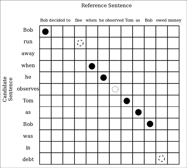
Figure 11.10: The METEOR word matching table

You can see that we denoted matches between the candidate sentence and the reference sentence in circles and ovals. For example, we denote exact matches with a solid black circle, synonyms with a dashed hollow circle, and stemmed matches with dotted circles.

METEOR is computationally more complex, but has often been found to correlate with human judgment more than BLEU, suggesting that METEOR is a better evaluation metric than BLEU.

CIDEr

Consensus-based Image Description Evaluation (CIDEr), proposed by Ramakrishna Vedantam and others in CIDEr: Consensus-based Image Description Evaluation, IEEE Conference on Computer Vision and Pattern Recognition (CVPR), 2015, is another measure that evaluates the consensus of a candidate sentence to a given set of reference statements. CIDEr is defined to measure the grammaticality, saliency, and accuracy (that is, precision and recall) of a candidate sentence.

First, CIDEr weighs each n-gram found in both the candidate and reference sentences by means of TF-IDF, so that more common n-grams (for example, the words a and the) will have a smaller weight, whereas rare words will have a higher weight. Finally, CIDEr is calculated as the cosine similarity between the vectors formed by TF-IDF-weighted n-grams found in the candidate sentence and the reference sentence:

Here, cand is the candidate sentence, ref is the set of reference sentences, ref_j is the j^th sentence of ref, and m is the number of reference sentences for a given candidate. Most importantly, is the TF-IDF values calculated for all the n-grams in the candidate sentence and formed as a vector. is the same vector for the reference sentence, ref_i. denotes the magnitude of the vector.

Overall, it should be noted that there is no clear-cut winner that is able to perform well across all the different tasks that are found in NLP. These metrics are significantly task-dependent and should be carefully chosen depending on the task. Here we’ll be using the BLEU score for our model.

Evaluating the model

With the model trained, let’s test the model on our unseen test dataset. Testing logic is almost identical to the validation logic we discussed earlier during model training. Therefore we will not repeat our discussion here.

bleu_metric = BLEUMetric(tokenizer=tokenizer)
test_dataset, _ = generate_tf_dataset(
    test_captions_df, tokenizer=tokenizer, n_vocab=n_vocab, batch_size=batch_size, training=False
)
test_loss, test_accuracy, test_bleu = [], [], []
for ti, t_batch in enumerate(test_dataset):
    print(f"{ti+1} batches processed", end='
')
    loss, accuracy = full_model.test_on_batch(t_batch[0], t_batch[1])
    batch_predicted = full_model.predict_on_batch(t_batch[0])
    bleu_score = bleu_metric.calculate_bleu_from_predictions(t_batch[1], batch_predicted)
    test_loss.append(loss)
    test_accuracy.append(accuracy)
    test_bleu.append(bleu_score)
print(
    f"
test_loss: {np.mean(test_loss)} - test_accuracy: {np.mean(test_accuracy)} - test_bleu: {np.mean(test_bleu)}"
)

This will output:

261 batches processed
test_loss: 1.057080413646625 - test_accuracy: 0.7914185857407434 - test_bleu: 0.10505496256163914

Great, we can see the model is showing a similar performance to what it did on the validation data. This means our model has not overfitted data, and should perform reasonably well in the real world. Let’s now generate captions for a few sample images.

Captions generated for test images

With the help of metrics such as accuracy and BLEU, we have ensured our model is performing well. But, one of the most important tasks a trained model has to perform is generating outputs for new data. We will learn how we can use our model to generate actual captions. Let’s first understand how we can generate captions at a conceptual level. It’s quite straightforward to generate the image representation using an image. The tricky part is adapting the text decoder to generate captions. As you can imagine, the decoder inference needs to work in a different setting than the training. This is because at inference we don’t have caption tokens to input to the model.

The way we predict with our model is by starting with the image and a starting caption that has the single token [START]. We feed these two inputs to the model to generate the next token. We then combine the new token with the current input and predict the next token. We keep going this way until we reach a certain number of steps or the model outputs [END] (Figure 11.11). If you remember, we developed the model in a way that it can accept an arbitrary length token sequence. This is extremely helpful during inference as at each time step, the length of the sequence increases.

Figure 11.11: How the decoder of the trained model is used to generate a new caption for a given image

We will choose a small dataset of 10 samples from the test dataset and generate captions:

n_samples = 10
test_dataset, _ = generate_tf_dataset(
    test_captions_df.sample(n=n_samples), tokenizer=tokenizer, 
    n_vocab=n_vocab, batch_size=n_samples, training=False
)

Next let’s define a function called generate_captions(). This function takes in:

• model – The trained model
• image_input – A batch of input images
• tokenizer – Trained tokenizer
• n_samples – Number of samples in the batch

As we can see in the following:

def generate_caption(model, image_input, tokenizer, n_samples):
    # 2 -> [START]
    batch_tokens = np.repeat(np.array([[2]]), n_samples, axis=0)
    
    for i in range(30):
        if np.all(batch_tokens[:,-1] == 3):
            break
            
        position_input = tf.repeat(tf.reshape(tf.range(i+1),[1,-1]), 
        n_samples, axis=0)
        probs = full_model((image_input, batch_tokens, 
        position_input)).numpy()
        batch_tokens = np.argmax(probs, axis=-1)
    
    predicted_text = []
    for sample_tokens in batch_tokens:
        sample_predicted_token_ids = sample_tokens.ravel()
        sample_predicted_tokens = []
        for wid in sample_predicted_token_ids:
            sample_predicted_tokens.append(tokenizer.id_to_token(wid))
            if wid == 3:
                break
        sample_predicted_text = " ".join([tok for tok in 
        sample_predicted_tokens])
        sample_predicted_text = sample_predicted_text.replace(" ##", 
        "")
        predicted_text.append(sample_predicted_text)
    
    return predicted_text

This function starts with a single caption token ID. The ID 2 maps to the token [START]. We predict for 30 steps or if the last token is [END] (mapped to token ID 3). We generate position inputs for the batch of data by creating a range sequence from 0 to i and repeating that n_sample times across the batch dimension. We then predict the token probabilities by feeding the inputs to the model.

We can now use this function to generate captions:

for batch in test_dataset.take(1):
    (batch_image_input, _, _), batch_true_caption = batch
batch_predicted_text = generate_caption(full_model, batch_image_input, tokenizer, n_samples)

Let’s now visualize the captions side by side with the image inputs. Additionally, we’ll show the ground truth captions:

fig, axes = plt.subplots(n_samples, 2, figsize=(8,30))
for i,(sample_image_input, sample_true_caption, sample_predicated_caption) in enumerate(zip(batch_image_input, batch_true_caption, batch_predicted_text)):
    
    sample_true_caption_tokens  = [tokenizer.id_to_token(wid) for wid in
    sample_true_caption.numpy().ravel()]
    
    sample_true_text = []
    for tok in sample_true_caption_tokens:
        sample_true_text.append(tok)
        if tok == '[END]':
            break
    
    sample_true_text = " ".join(sample_true_text).replace(" ##", "")
    axes[i][0].imshow(((sample_image_input.numpy()+1.0)/2.0))
    axes[i][0].axis('off')
    
    true_annotation = f"TRUE: {sample_true_text}"
    predicted_annotation = f"PRED: {sample_predicated_caption}"
    axes[i][1].text(0, 0.75, true_annotation, fontsize=18)
    axes[i][1].text(0, 0.25, predicted_annotation, fontsize=18)
    axes[i][1].axis('off')

You will get a plot similar to the following. The images sampled will be randomly sampled every time it runs. The results of this run can be seen in Figure 11.12:

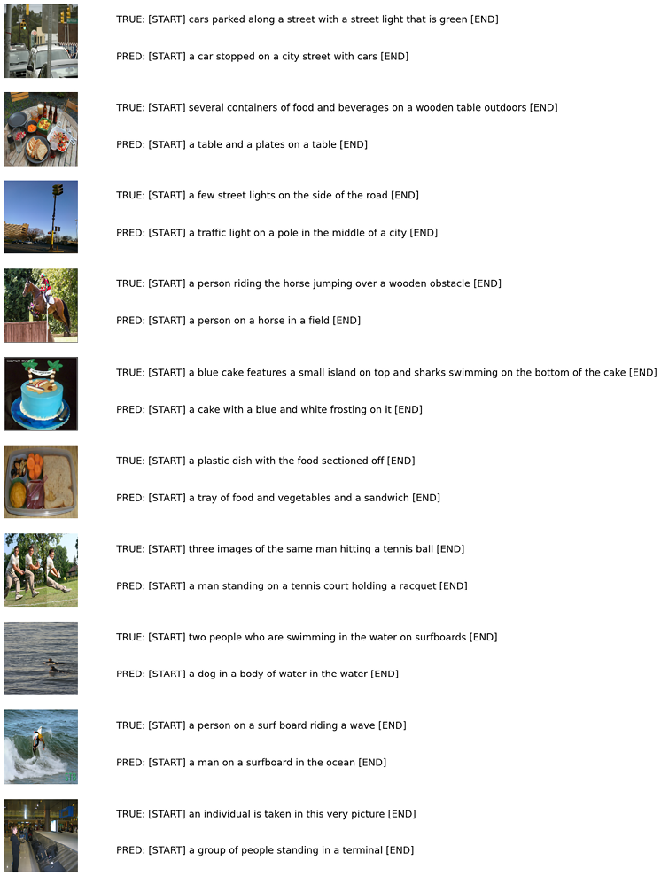
Figure 11.12: Captions generated on a sample of test data

We can see that our model does a good job of generating captions. In general, we can see that the model can identify objects and activities portrayed in the images. It is also important to remember that each of our images has multiple captions associated with it. Therefore, the predicted captions do not necessarily need to match the ground truth caption shown in the image.

Summary

In this chapter, we focused on a very interesting task that involves generating captions for given images. Our image-captioning model was one of the most complex models in this book, which included the following:

• A vision Transformer model that produces an image representation
• A text-based Transformer decoder

Before we began with the model, we analyzed our dataset to understand various characteristics such as image sizes and the vocabulary size. Then we understood how we can use a tokenizer to tokenize captions strings. We then used this knowledge to build a TensorFlow data pipeline.

We discussed each component in detail. The Vision Transformer (ViT) takes in an image and produces a hidden representation of that image. Specifically, the ViT breaks an image into a sequence of 16x16 patches of pixels. After that, it treats each patch as a token embedding to the Transformer (along with positional information) to produce a representation of each patch. It also incorporates the [CLS] token at the beginning to provide a holistic representation of the image.

Next the text decoder takes in the image representation along with caption tokens as inputs. The objective of the decoder becomes to predict the next token at each time step. We were able to reach a BLEU-4 score of just above 0.10 for the validation dataset.

Thereafter, we discussed several different metrics (BLEU, ROUGE, METEOR, and CIDEr), which we can use to quantitatively evaluate the generated captions, and we saw that as we ran our algorithm through the training data, the BLEU-4 score increased over time. Additionally, we visually inspected the generated captions and saw that our ML pipeline progressively gets better at captioning images.

Next, we evaluated our model on the test dataset and validated that it demonstrates similar performance on test data as expected. Finally, we learned how we can use the trained model to generate captions for unseen images.

We have reached the end of the book. We have covered many different topics in natural language and discussed state-of-the-art models and techniques that help us to solve problems.

In the Appendix, we will discuss some mathematical concepts related to machine learning, followed by an explanation of how to use the visualization tool TensorBoard to visualize word vectors.

To access the code files for this book, visit our GitHub page at: https://packt.link/nlpgithub

Join our Discord community to meet like-minded people and learn alongside more than 1000 members at: https://packt.link/nlp