9

Sequence-to-Sequence Learning – Neural Machine Translation

Sequence-to-sequence learning is the term used for tasks that require mapping an arbitrary-length sequence to another arbitrary-length sequence. This is one of the most sophisticated tasks in NLP, which involves learning many-to-many mappings. Examples of this task include Neural Machine Translation (NMT) and creating chatbots. NMT is where we translate a sentence from one language (source language) to another (target language). Google Translate is an example of an NMT system. Chatbots (that is, software that can communicate with/answer a person) are able to converse with humans in a realistic manner. This is especially useful for various service providers, as chatbots can be used to find answers to easily solvable questions that customers might have, instead of redirecting them to human operators.

In this chapter, we will learn how to implement an NMT system. However, before diving directly into such recent advances, we will first briefly visit some Statistical Machine Translation (SMT) methods, which preceded NMT and were the state-of-the-art systems until NMT caught up. Next, we will walk through the steps required for building an NMT. Finally, we will learn how to implement a real NMT system that translates from German to English, step by step.

Specifically, this chapter will cover the following main topics:

• Machine translation
• A brief historical tour of machine translation
• Understanding neural machine translation
• Preparing data for the NMT system
• Defining the model
• Training the NMT
• The BLEU score – evaluating the machine translation systems
• Visualizing attention patterns
• Inference with NMT
• Other applications of Seq2Seq models – chatbots

Machine translation

Humans often communicate with each other by means of a language, compared to other communication methods (for example, gesturing). Currently, more than 6,000 languages are spoken worldwide. Furthermore, learning a language to a level where it is easily understandable to a native speaker of that language is a difficult task to master. However, communication is essential for sharing knowledge, socializing, and expanding your network. Therefore, language acts as a barrier to communicating with people in different parts of the world. This is where Machine Translation (MT) comes in. MT systems allow the user to input a sentence in their own tongue (known as the source language) and output a sentence in a desired target language.

The problem with MT can be formulated as follows. Say we are given a sentence (or a sequence of words) W_s belonging to a source language S, defined by the following:

Here, .

The source language would be translated to a sentence , where T is the target language and is given by the following:

Here, .

is obtained through the MT system, which outputs the following:

Here, is the pool of possible translation candidates found by the algorithm for the source sentence. Also, the best candidate from the pool of candidates is given by the following equation:

Here, is the model parameters. During training, we optimize the model to maximize the probability of some known target translations for a set of corresponding source translations (that is, training data).

So far, we have discussed the formal setup of the language translation problem that we’re interested in solving. Next, we will walk through the history of MT to get a feel of how people tried solving this in the early days.

A brief historical tour of machine translation

Here, we will discuss the history of MT. The inception of MT involved rule-based systems. Then, more statistically sound MT systems emerged. Statistical Machine Translation (SMT) used various measures of statistics of a language to produce translations to another language. Then came the era of NMT. NMT currently holds state-of-the-art performance in most machine learning tasks compared with other methods.

Rule-based translation

NMT came long after statistical machine learning, and statistical machine learning has been around for more than half a century now. The inception of SMT methods dates back to 1950-60, when during one of the first recorded projects, the Georgetown-IBM experiment, more than 60 Russian sentences were translated to English. o give some perspective, this attempt is almost as old as the invention of the transistor.

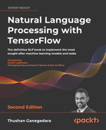
One of the initial techniques for MT was word-based machine translation. This system performed word-to-word translations using bilingual dictionaries. However, as you can imagine, this method has serious limitations. The obvious limitation is that word-to-word translation is not a one-to-one mapping between different languages. In addition, word-to-word translation may lead to incorrect results as it does not consider the context of a given word. The translation of a given word in the source language can change depending on the context in which it is used. To understand this with a concrete example, let’s look at the translation example from English to French in Figure 9.1. You can see that in the given two English sentences, a single word changes. However, this creates drastic changes in the translation:

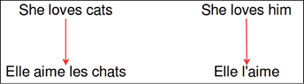
Figure 9.1: Translations (English to French) between languages are not one-to-one mappings between words

In the 1960s, the Automatic Language Processing Advisory Committee (ALPAC) released a report, Languages and machines: computers in translation and linguistics, National Academy of the Sciences (1966), on MT’s prospects. The conclusion was this:

There is no immediate or predictable prospect of useful machine translation.

This was because MT was slower, less accurate, and more expensive than human translation at the time. This delivered a huge blow to MT advancements, and almost a decade passed in silence.

Next came corpora-based MT, where an algorithm was trained using tuples of source sentences, and the corresponding target sentence was obtained through a parallel corpus, that is, the parallel corpus would be of the format [(<source_sentence_1>, <target_sentence_1>), (<source_sentence_2>, <target_sentence_2>), …]. The parallel corpus is a large text corpus formed as tuples, consisting of text from the source language and the corresponding translation of that text. An illustration of this is shown in Table 9.1. It should be noted that building a parallel corpus is much easier than building bilingual dictionaries and they are more accurate because the training data is richer than word-to-word training data. Furthermore, instead of directly relying on manually created bilingual dictionaries, a bilingual dictionary (that is, the transition models) of two languages can be built using the parallel corpus. A transition model shows how likely a target word/phrase is to be the correct translation, given the current source word/phrase. In addition to learning the transition model, corpora-based MT also learns the word alignment models. A word alignment model can represent how words in a phrase from the source language correspond to the translation of that phrase. An example of parallel corpora and a word alignment model is depicted in Figure 9.2:

Figure 9.2: Word alignment between two different languages

An illustration of an example parallel corpora is shown in Table 9.1:

Table 9.1: Parallel corpora for English and French sentences

Another approach was interlingual machine translation, which involved translating the source sentence into a language-neutral interlingua (that is, a metalanguage), and then generating the translated sentence out of the interlingua. More specifically, an interlingual machine translation system consists of two important components, an analyzer and a synthesizer. The analyzer will take the source sentence and identify agents (for example, nouns), actions (for example, verbs), and so on, and also how they interact with each other. Next, these identified elements are represented by means of an interlingual lexicon. An example of an interlingual lexicon can be made with the synsets (that is, the group of synonyms sharing a common meaning) available in WordNet. Then, from this interlingual representation, the synthesizer will create the translation. Since the synthesizer knows the nouns, verbs, and so on through the interlingual representation, it can generate the translation in the target language by incorporating language-specific grammar rules.

Statistical Machine Translation (SMT)

Next, more statistically sound systems started emerging. One of the pioneering models of this era was IBM Models 1-5, which did word-based translation. However, as we discussed earlier, word translations do not match one to one from the source language to a target language (for example, compound words and morphology). Eventually, researchers started experimenting with phrase-based translation systems, which made some notable advances in machine translation.

Phrase-based translation works in a similar way to word-based translation, except that it uses phrases of a language as the atomic units of translation instead of individual words. This is a more sensible approach as it makes modeling the one-to-many, many-to-one, or many-to-many relationships between words easier. The main goal of phrase-based translation is to learn a phrase-translation model that contains a probability distribution of different candidate target phrases for a given source phrase. As you can imagine, this method involves maintaining huge databases of various phrases in two languages. A reordering step for phrases is also performed as there is no monotonic ordering of words between a sentence from one language and one in another.

An example of this is shown in Figure 9.2; if the words were monotonically ordered between languages, there would not be crosses between word mappings.

One of the limitations of this approach is that the decoding process (finding the best target phrase for a given source phrase) is expensive. This is due to the size of the phrase database, as well as the fact that a source phrase often contains multiple target language phrases. To alleviate the burden, syntax-based translations arose.

In syntax-based translation, the source sentence is represented by a syntax tree. In Figure 9.3, NP represents a noun phrase, VP a verb phrase, and S a sentence. Then a reordering phase takes place, where the tree nodes are reordered to change the order of subject, verb, and object, depending on the target language. This is because the sentence structure can change depending on the language (for example, in English it is subject-verb-object, whereas in Japanese it is subject-object-verb). The reordering is decided according to something known as the r-table. The r-table contains the likelihood probabilities for the tree nodes to be changed to some other order:

Figure 9.3: Syntax tree for a sentence

An insertion phase then takes place. In the insertion phase, we stochastically insert a word into each node of the tree. This is due to the assumption that there is an invisible NULL word, and it generates target words at random positions of the tree. Also, the probability of inserting a word is determined by something called the n-table, which is a table that contains probabilities of inserting a particular word into the tree.

Next, the translation phase occurs, where each leaf node is translated to the target word in a word-by-word manner. Finally, the translated sentence is read off the syntax tree, to construct the target sentence.

Neural Machine Translation (NMT)

Finally, around the year 2014, NMT systems were introduced. NMT is an end-to-end system that takes a full sentence as an input, performs certain transformations, and then outputs the translated sentence for the corresponding source sentence.

Therefore, NMT eliminates the need for the feature engineering required for machine translation, such as building phrase translation models and building syntax trees, which is a big win for the NLP community. Also, NMT has outperformed all the other popular MT techniques in a very short period, just two to three years. In Figure 9.4, we depict the results of various MT systems reported in the MT literature. For example, 2016 results are obtained from Sennrich and others in their paper Edinburgh Neural Machine Translation Systems for WMT 16, Association for Computational Linguistics, Proceedings of the First Conference on Machine Translation, August 2016: 371-376, and from Williams and others in their paper Edinburgh’s Statistical Machine Translation Systems for WMT16, Association for Computational Linguistics, Proceedings of the First Conference on Machine Translation, August 2016: 399-410. All the MT systems are evaluated with the BLEU score. The BLEU score denotes the number of n-grams (for example, unigrams and bigrams) of candidate translation that matched in the reference translation. So the higher the BLEU score, the better the MT system. We’ll discuss the BLEU metric in detail later in the chapter. There is no need to highlight that NMT is a clear-cut winner:

Figure 9.4: Comparison of statistical machine translation system to NMT systems. Courtesy of Rico Sennrich

A case study assessing the potential of NMT systems is available in Is Neural Machine Translation Ready for Deployment? A Case Study on 30 Translation Directions, Junczys-Dowmunt, Hoang and Dwojak, Proceedings of the Ninth International Workshop on Spoken Language Translation, Seattle (2016).

The study looks at the performance of different systems on several translation tasks between various languages (English, Arabic, French, Russian, and Chinese). The results also support that NMT systems (NMT 1.2M and NMT 2.4M) perform better than SMT systems (PB-SMT and Hiero).

Figure 9.5 shows several statistics for a set from a 2017 state-of-the-art machine translator. This is from a presentation, State of the Machine Translation, Intento, Inc, 2017, produced by Konstantin Savenkov, cofounder and CEO of Intento. We can see that the performance of the MT produced by DeepL (https://www.deepl.com) appears to be competing closely with other MT giants, including Google. The comparison includes MT systems such as DeepL (NMT), Google (NMT), Yandex (NMT-SMT hybrid), Microsoft (has both SMT and NMT), IBM (SMT), Prompt (rule-based), and SYSTRAN (rule-based/SMT hybrid). The graph clearly shows that NMT systems are leading the current MT advancements. The LEPOR score is used to assess different systems. LEPOR is a more advanced metric than BLEU, and it attempts to solve the language bias problem. The language bias problem refers to the phenomenon that some evaluation metrics (such as BLEU) perform well for certain languages, but perform poorly for others.

However, it should also be noted that the results do contain some bias due to the averaging mechanism used in this comparison. For example, Google Translate has been averaged over a larger set of languages (including difficult translation tasks), whereas DeepL has been averaged over a smaller and relatively easier subset of languages. Therefore, we should not conclude that the DeepL MT system is always better than the Google MT system. Nevertheless, the overall results provide a general comparison of the performance of the current NMT and SMT systems:

Figure 9.5: Performance of various MT systems. Courtesy of Intento, Inc.

We saw that NMT has already outperformed SMT systems in very few years, and is the current state of the art. We will now move on to discussing the details and architecture of an NMT system. Finally, we will be implementing an NMT system from scratch.

Understanding neural machine translation

Now that we have an appreciation for how machine translation has evolved over time, let’s try to understand how state-of-the-art NMT works. First, we will take a look at the model architecture used by neural machine translators and then move on to understanding the actual training algorithm.

Intuition behind NMT systems

First, let’s understand the intuition underlying an NMT system’s design. Say you are a fluent English and German speaker and were asked to translate the following sentence into German:

I went home

This sentence translates to the following:

Ich ging nach Hause

Although it might not have taken more than a few seconds for a fluent person to translate this, there is a certain process that produces the translation. First, you read the English sentence, and then you create a thought or concept about what this sentence represents or implies, in your mind. And finally, you translate the sentence into German. The same idea is used for building NMT systems (see Figure 9.6). The encoder reads the source sentence (that is, similar to you reading the English sentence). Then the encoder outputs a context vector (the context vector corresponds to the thought/concept you imagined after reading the sentence). Finally, the decoder takes in the context vectors and outputs the translation in German:

Figure 9.6: Conceptual architecture of an NMT system

NMT architecture

Now we will look at the architecture in more detail. The sequence-to-sequence approach was originally proposed by Sutskever, Vinyals, and Le in their paper Sequence to Sequence Learning with Neural Networks, Proceedings of the 27th International Conference on Neural Information Processing Systems - Volume 2: 3104-3112.

From the diagram in Figure 9.6, we can see that there are two major components in the NMT architecture. These are called the encoder and decoder. In other words, NMT can be seen as an encoder-decoder architecture. The encoder converts a sentence from a given source language into a thought vector (i.e. a contextualized representation), and the decoder decodes or translates the thought into a target language. As you can see, this shares some features with the interlingual machine translation method we briefly talked about. This explanation is illustrated in Figure 9.7. The left-hand side of the context vector denotes the encoder (which takes a source sentence in word by word to train a time-series model). The right-hand side denotes the decoder, which outputs word by word (while using the previous word as the current input) the corresponding translation of the source sentence. We will also use embedding layers (for both the source and target languages) where the semantics of the individual tokens will be learned and fed as inputs to the models:

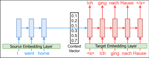
Figure 9.7: Unrolling the source and target sentences over time

With a basic understanding of what NMT looks like, let’s formally define the objective of the NMT. The ultimate objective of an NMT system is to maximize the log likelihood, given a source sentence x_s and its corresponding y_t. That is, to maximize the following:

Here, N refers to the number of source and target sentence inputs we have as training data.

Then, during inference, for a given source sentence, , we will find the translation using the following:

Here, is the predicted token at the i^th time step and is the set of possible candidate sentences.

Before we examine each part of the NMT architecture, let’s define the mathematical notation to understand the system more concretely. As our sequential model, we will choose a Gated Recurrent Unit (GRU), as it is simpler than an LSTM and performs comparatively well.

Let’s define the encoder GRU as and the decoder GRU as . At the time step , let’s define the output state of a general GRU as h_t. That is, feeding the input x_t into the GRU produces h_t:

Now, we will talk about the embedding layer, the encoder, the context vector, and finally, the decoder.

The embedding layer

We have already seen the power of word embeddings. Here, we can also leverage embeddings to improve model performance. We will be using two-word embedding layers, , for the source language and for the target language. So, instead of feeding x_t directly into the GRU, we will be getting . However, to avoid excessive notation, we will assume .

The encoder

As mentioned earlier, the encoder is responsible for generating a thought vector or a context vector that represents what is meant by the source language. For this, we will use a GRU-based network (see Figure 9.8):

Figure 9.8: A GRU cell

The encoder is initialized with h at time step 0 (h₀) with a zero vector by default. The encoder takes a sequence of words, , as the input and calculates a context vector, , where v is the final external hidden state obtained after processing the final element , of the sequence x_s. We represent this as the following:

The context vector

The idea of the context vector (v) is to represent a sentence of a source language concisely. Also, in contrast to how the encoder’s state is initialized (that is, it is initialized with zeros), the context vector becomes the initial state for the decoder GRU. In other words, the decoder GRU doesn’t start with an initial state of zeros, but with the context vector as its initial state. This creates a linkage between the encoder and the decoder and makes the whole model end-to-end differentiable. We will talk about this in more detail next.

The decoder

The decoder is responsible for decoding the context vector into the desired translation. Our decoder is an RNN as well. Though it is possible for the encoder and decoder to share the same set of weights, it is usually better to use two different networks for the encoder and the decoder. This increases the number of parameters in our model, allowing us to learn the translations more effectively.

First, the decoder’s states are initialized with the context vector, i.e. , as shown here: .

Here, is the initial state vector of the decoder ().

This (v) is the crucial link that connects the encoder with the decoder to form an end-to-end computational chain (see in Figure 9.6 that the only thing shared by the encoder and decoder is v). Also, this is the only piece of information that is available to the decoder about the source sentence.

Then we will compute the m^th prediction of the translated sentence with the following:

The full NMT system with the details of how the GRU cell in the encoder connects to the GRU cell in the decoder, and how the softmax layer is used to output predictions, is shown in Figure 9.9:

Figure 9.9: The encoder-decoder architecture with the GRUs. Both the encoder and the decoder have a separate GRU component. Additionally, the decoder has a fully-connected (dense) layer and a softmax layer that produce the final predictions.

In the next section, we will go through the steps required to prepare data for our model.

Preparing data for the NMT system

In this section, we will understand the data and learn about the process for preparing data for training and predicting from the NMT system. First, we will talk about how to prepare training data (that is, the source sentence and target sentence pairs) to train the NMT system, followed by inputting a given source sentence to produce the translation of the source sentence.

The dataset

The dataset we’ll be using for this chapter is the WMT-14 English-German translation data from https://nlp.stanford.edu/projects/nmt/. There are ~4.5 million sentence pairs available. However, we will use only 250,000 sentence pairs due to computational feasibility. The vocabulary consists of the 50,000 most common English words and the 50,000 most common German words, and words not found in the vocabulary will be replaced with a special token, <unk>. You will need to download the following files:

• train.de – File containing German sentences
• train.en – File containing English sentences
• vocab.50K.de – File containing German vocabulary
• vocab.50K.en – File containing English vocabulary

train.de and train.en contain parallel sentences in German and English, respectively. Once downloaded we will load the sentences as follows:

n_sentences = 250000
# Loading English sentences
original_en_sentences = []
with open(os.path.join('data', 'train.en'), 'r', encoding='utf-8') as en_file:
    for i,row in enumerate(en_file):
        if i >= n_sentences: break
        original_en_sentences.append(row.strip().split(" "))
        
# Loading German sentences
original_de_sentences = []
with open(os.path.join('data', 'train.de'), 'r', encoding='utf-8') as de_file:
    for i, row in enumerate(de_file):
        if i >= n_sentences: break
        original_de_sentences.append(row.strip().split(" "))

If you print the data you just loaded, for the two languages, you would have sentences like the following:

English: a fire restant repair cement for fire places , ovens , open fireplaces etc . 
German: feuerfester Reparaturkitt für Feuerungsanlagen , Öfen , offene Feuerstellen etc.
English: Construction and repair of highways and ... 
German: Der Bau und die Reparatur der Autostraßen ...
English: An announcement must be commercial character . 
German: die Mitteilungen sollen den geschäftlichen kommerziellen Charakter tragen .

Adding special tokens

The next step is to add a few special tokens to the start and end of our sentences. We will add <s> to mark the start of a sentence and </s> to mark the end of a sentence. We can easily achieve this using the following list comprehension:

en_sentences = [["<s>"]+sent+["</s>"] for sent in original_en_sentences]
de_sentences = [["<s>"]+sent+["</s>"] for sent in original_de_sentences]

This will give us:

English: <s> a fire restant repair cement for fire places , ovens , open fireplaces etc . </s> 
German: <s> feuerfester Reparaturkitt für Feuerungsanlagen , Öfen , offene Feuerstellen etc. </s>
English: <s> Construction and repair of highways and ... </s> 
German: <s> Der Bau und die Reparatur der Autostraßen ... </s>
English: <s> An announcement must be commercial character . </s> 
German: <s> die Mitteilungen sollen den geschäftlichen kommerziellen Charakter tragen . </s>

This is a very important step for Seq2Seq models. <s> and </s> tokens serve an extremely important role during model inference. As you will see, at inference time, we will be using the decoder to predict one word at a time, by using the output of the previous time step as an input. This way we can predict for an arbitrary number of time steps. Using <s> as the starting token gives us a way to signal to the decoder that it should start predicting tokens from the target language. Next, if we do not use the </s> token to mark the end of a sentence, we cannot signal the decoder to end a sentence. This can lead the model to enter an infinite loop of predictions.

Splitting training, validation, and testing datasets

We need to split our dataset into three parts: a training set, a validation set, and a testing set. Specifically, let’s use 80% of sentences to train the model, 10% as validation data, and the remaining 10% as testing data:

from sklearn.model_selection import train_test_split
train_en_sentences, valid_test_en_sentences, train_de_sentences, valid_test_de_sentences = train_test_split(
    np.array(en_sentences), np.array(de_sentences), test_size=0.2
)
valid_en_sentences, valid_de_sentences, test_en_sentences, test_de_sentences = train_test_split(
    valid_test_en_sentences, valid_test_de_sentences, test_size=0.5)

Defining sequence lengths for the two languages

A key statistic we have to understand at this point is how long, generally, the sentences in our corpus are. It is quite likely that the two languages will have different sentence lengths. To learn the statistics of this, we’ll be using the pandas library in the following way:

pd.Series(train_en_sentences).str.len().describe(percentiles=[0.05, 0.5, 0.95])

Here, we are first converting the train_en_sentences to a pd.Series object. pd.Series is an indexed series of values (an array). Here, each value is a list of tokens belonging to each sentence. Calling .str.len() will give us the length of each list of tokens. Finally, the describe method will give important statistics such as mean, standard deviation, and percentiles. Here. we are specifically asking for 5%, 50%, and 95% percentiles.

Note that we are only using the training data for this calculation. If you include validation or test datasets in these calculations, we may be leaking data about validation and test data. Therefore, it’s best to only use the training dataset for these calculations.

The result from the previous code gives us:

Sequence lengths (English)
count    40000.000000
mean        25.162625
std         13.857748
min          6.000000
5%           9.000000
50%         22.000000
95%         53.000000
max        100.000000
dtype: float64

We can get the same for the German sentences the following way:

pd.Series(train_de_sentences).str.len().describe(percentiles=[0.05, 0.5, 0.95])

This gives us:

Sequence lengths (German)
count    40000.000000
mean        22.882550
std         12.574325
min          6.000000
5%           9.000000
50%         20.000000
95%         47.000000
max        100.000000
dtype: float64

Here we can see that 95% of English sentences have 53 tokens, where 95% of German sentences have 47 tokens.

Padding the sentences

Next, we need to pad our sentences. For this, we will use the pad_sequences() function provided in Keras. This function takes in values for the following arguments:

• sequences – A list of strings/IDs representing the text corpus. Each document can either be a list of strings or a list of integers
• maxlen – The maximum length to pad for (defaults to None)
• dtype – The type of data (defaults to 'int32')
• padding – The side to pad short sequences (defaults to 'pre')
• truncating – The side to truncate long sequences from (defaults to 'pre')
• value – The values to pad with (defaults to 0.0)

We will use this function as follows:

from tensorflow.keras.preprocessing.sequence import pad_sequences
train_en_sentences_padded = pad_sequences(train_en_sentences, maxlen=n_en_seq_length, value=unk_token, dtype=object, truncating='post', padding='post')
valid_en_sentences_padded = pad_sequences(valid_en_sentences, maxlen=n_en_seq_length, value=unk_token, dtype=object, truncating='post', padding='post')
test_en_sentences_padded = pad_sequences(test_en_sentences, maxlen=n_en_seq_length, value=unk_token, dtype=object, truncating='post', padding='post')
train_de_sentences_padded = pad_sequences(train_de_sentences, maxlen=n_de_seq_length, value=unk_token, dtype=object, truncating='post', padding='post')
valid_de_sentences_padded = pad_sequences(valid_de_sentences, maxlen=n_de_seq_length, value=unk_token, dtype=object, truncating='post', padding='post')
test_de_sentences_padded = pad_sequences(test_de_sentences, maxlen=n_de_seq_length, value=unk_token, dtype=object, truncating='post', padding='post')

We are padding all of the training, validation, and test sentences in both English and German. We will use the recently found sequence lengths as the padding/truncating length.

Next let’s define our encoder-decoder model.

Defining the model

In this section, we will define the model from end to end.

We are going to implement an encoder-decoder based NMT model equipped with additional techniques to boost performance. Let’s start off by converting our string tokens to IDs.

Converting tokens to IDs

Before we jump to the model, we have one more text processing operation remaining, that is, converting the processed text tokens into numerical IDs. We are going to use a tf.keras.layers.Layer to do this. Particularly, we’ll be using the StringLookup layer to create a layer in our model that converts each token into a numerical ID. As the first step, let us load the vocabulary files provided in the data. Before doing so, we will define the variable n_vocab to denote the size of the vocabulary for each language:

n_vocab = 25000 + 1

Originally, each vocabulary contains 50,000 tokens. However, we’ll take only half of this to reduce the memory requirement. Note that we allow one extra token as there’s a special token <unk> to denote out-of-vocabulary (OOV) words. With a 50,000-token vocabulary, it is quite easy to run out of memory due to the size of the final prediction layer we’ll build. While cutting back on the size of the vocabulary, we have to make sure that we preserve the most common 25,000 words. Fortunately, each vocabulary file is organized such that words are ordered by their frequency of occurrence (high to low). Therefore, we just need to read the first 25,001 lines of text from the file:

en_vocabulary = []
with open(os.path.join('data', 'vocab.50K.en'), 'r', encoding='utf-8') as en_file:
    for ri, row in enumerate(en_file):
        if ri  >= n_vocab: break
        
        en_vocabulary.append(row.strip())

Then we do the same for the German vocabulary:

de_vocabulary = []
with open(os.path.join('data', 'vocab.50K.de'), 'r', encoding='utf-8') as de_file:
    for ri, row in enumerate(de_file):
        if ri >= n_vocab: break
        
        de_vocabulary.append(row.strip())

Each of the vocabularies contain the special OOV token <unk> as the first line. We’ll pop that out of the en_vocabulary and de_vocabulary lists as we need this for the next step:

en_unk_token = en_vocabulary.pop(0)
de_unk_token = de_vocabulary.pop(0)

Here’s how we can define our English StringLookup layer:

en_lookup_layer = tf.keras.layers.StringLookup(
    vocabulary=en_vocabulary, oov_token=en_unk_token, 
    mask_token=pad_token, pad_to_max_tokens=False
)

Let’s understand the arguments provided to this layer:

• vocabulary – Contains a list of words that are found in the corpus (except certain special tokens that will be discussed below)
• oov_token – A special out-of-vocabulary token that will be used to replace tokens not listed in the vocabulary
• mask_token – A special token that will be used to mask inputs (e.g. uninformative padded tokens)
• pad_to_max_tokens – If padding should occur to bring arbitrary-length sequences in a batch of data to the same length

Similarly, we define a lookup layer for the German language:

de_lookup_layer = tf.keras.layers.StringLookup(
    vocabulary=de_vocabulary, oov_token=de_unk_token, 
    mask_token=pad_token, pad_to_max_tokens=False
)

With the groundwork laid out, we can start building the encoder.

Defining the encoder

We start the encoder with an input layer. The input layer will take in a batch of sequences of tokens. Each sequence of tokens is n_en_seq_length elements long. Remember that we padded or truncated the sentences to make sure all of them have a fixed length of n_en_seq_length:

encoder_input = tf.keras.layers.Input(shape=(n_en_seq_length,), dtype=tf.string)

Next we use the previously defined StringLookup layer to convert the string tokens into word IDs. As we saw, the StringLookup layer can take a list of unique words (i.e. a vocabulary) and create a lookup operation to convert a given token into a numerical ID:

encoder_wid_out = en_lookup_layer(encoder_input)

With the tokens converted into IDs, we route the generated word IDs to a token embedding layer. We pass in the size of the vocabulary (derived from the en_lookup_layer's get_vocabulary() method) and the embedding size (128) and finally we ask the layer to mask any zero-valued inputs as they don’t contain any information:

en_full_vocab_size = len(en_lookup_layer.get_vocabulary())
encoder_emb_out = tf.keras.layers.Embedding(en_full_vocab_size, 128, mask_zero=True)(encoder_wid_out)

The output of the embedding layer is stored in encoder_emb_out. Next we define a GRU layer to process the sequence of English token embeddings:

encoder_gru_out, encoder_gru_last_state = tf.keras.layers.GRU(256, return_sequences=True, return_state=True)(encoder_emb_out)

Note how we are setting both the return_sequences and return_state arguments to True. To recap, return_sequences returns the full sequence of hidden states as the output (instead of returning only the last), where return_state returns the last state of the model as an additional output. We need both these outputs to build the rest of our model. For example, we need to pass the last state of the encoder to the decoder as the initial state. For that, we need the last state of the encoder (stored in encoder_gru_last_state). We will discuss the purpose of this in more detail as we go. We now have everything to define the encoder part of our model. It takes in a batch of sequences of string tokens and returns the full sequence of GRU hidden states as the output.

encoder = tf.keras.models.Model(inputs=encoder_input, outputs=encoder_gru_out)

With the encoder defined, let’s build the decoder.

Defining the decoder

Our decoder will be more complex than the encoder. The objective of the decoder is, given the last encoder state and the previous token the decoder predicted, predict the next token. For example, for the German sentence:

<s> ich ging zum Laden </s>

We define:

This technique is known as teacher forcing. In other words, the decoder is leveraging previous tokens of the target itself to predict the next token. This makes the translation task easier for the model. We can understand this phenomenon as follows. Say a teacher asks a kindergarten student to complete the following sentence, given just the first word:

I ___ ____ ___ ___ ____ ____

This means that the child needs to pick a subject, verb, and object; know the syntax of the language; understand the grammar rules of the language; and so on. Therefore, the likelihood of the child producing an incorrect sentence is high.

However, if we ask the child to produce it word by word, they might do a better job at coming up with a sentence. In other words, we ask the child to produce the next word given the following:

I ____

Then we ask them to fill in the blank given:

I like ____

And continue in the same fashion:

I like to ___, I like to fly ____, I like to fly kites ____

This way, the child can do a better job at producing a correct and meaningful sentence. We can adopt the same approach to alleviate the difficulty of the translation task, as shown in Figure 9.10:

Figure 9.10: The teacher forcing mechanism. The darker arrows in the inputs depict newly introduced input connections to the decoder. The right-hand side figure shows how the decoder GRU cell changes.

To feed in previous tokens predicted by the decoder, we need an input layer for the decoder. When formulating the decoder inputs and outputs this way, for a sequence of tokens with length n, the input and output are n-1 tokens long:

decoder_input = tf.keras.layers.Input(shape=(n_de_seq_length-1,), dtype=tf.string)

Next, we use the de_lookup_layer defined earlier to convert tokens to IDs:

decoder_wid_out = de_lookup_layer(decoder_input)

Similar to the encoder, let’s define an embedding layer for the German language:

de_full_vocab_size = len(de_lookup_layer.get_vocabulary())
decoder_emb_out = tf.keras.layers.Embedding(de_full_vocab_size, 128, mask_zero=True)(decoder_wid_out)

We define a GRU layer in the decoder that will take the token embeddings and produce hidden outputs:

decoder_gru_out = tf.keras.layers.GRU(256, return_sequences=True)(decoder_emb_out, initial_state=encoder_gru_last_state)

Note that we are passing the encoder’s last state to a special argument called initial_state in the GRU’s call() method. This ensures that the decoder uses the encoder’s last state to initialize its memory.

The next step of our journey takes us to one of the most important concepts in machine learning, ‘attention.’ So far, the decoder had to rely on the encoder’s last state as the ‘only’ input/signal about the source language. This is like asking to summarize a sentence using a single word. Generally, when doing so, you lose a lot of the meaning and message in this conversion. Attention alleviates this problem.

Attention: Analyzing the encoder states

Instead of relying just on the encoder’s last state, attention enables the decoder to analyze the complete history of state outputs. The decoder does this at every step of the prediction and creates a weighted average of all the state outputs depending on what it needs to produce at that step. For example, in the translation I went to the shop -> ich ging zum Laden, when predicting the word ging, the decoder will pay more attention to the first part of the English sentence than the latter.

There have been many different implementations of attention over the years. It’s important to properly emphasize the need for attention in NMT systems. As you have learned previously, the context, or thought vector, that resides between the encoder and the decoder is a performance bottleneck (see Figure 9.11):

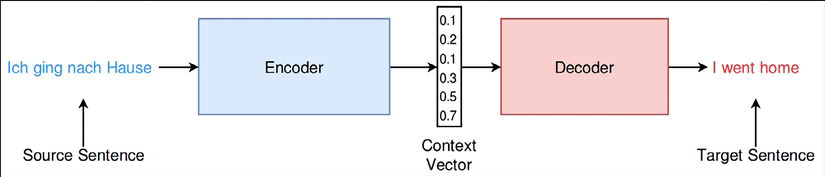
Figure 9.11: The encoder-decoder architecture

To understand why this is a bottleneck, let’s imagine translating the following English sentence:

I went to the flower market to buy some flowers

This translates to the following:

Ich ging zum Blumenmarkt, um Blumen zu kaufen

If we are to compress this into a fixed-length vector, the resulting vector needs to contain these:

• Information about the subject (I)
• Information about the verbs (buy and went)
• Information about the objects (flowers and flower market)
• Interaction of the subjects, verbs, and objects with each other in the sentence

Generally, the context vector has a size of 128 or 256 elements. Reliance on the context vector to store all this information with a small-sized vector is very impractical and an extremely difficult requirement for the system. Therefore, most of the time, the context vector fails to provide the complete information required to make a good translation. This results in an underperforming decoder that suboptimally translates a sentence.

To make the problem worse, during decoding the context vector is observed only in the beginning. Thereafter, the decoder GRU must memorize the context vector until the end of the translation. This becomes more and more difficult for long sentences.

Attention sidesteps this issue. With attention, the decoder will have access to the full state history of the encoder for each decoding time step. This allows the decoder to access a very rich representation of the source sentence. Furthermore, the attention mechanism introduces a softmax layer that allows the decoder to calculate a weighted mean of the past observed encoder states, which will be used as the context vector for the decoder. This allows the decoder to pay different amounts of attention to different words at different decoding steps.

Figure 9.12 shows a conceptual breakdown of the attention mechanism:

Figure 9.12: Conceptual attention mechanism in NMT

Next, let’s look at how we can compute attention.

Computing Attention

Now let’s investigate the actual implementation of the attention mechanism in detail. For this, we will use the Bahdanau attention mechanism introduced in the paper Neural Machine Translation by Learning to Jointly Align and Translate, by Bahdanau et al. We will discuss the original attention mechanism here. However, we’ll be implementing a slightly different version of it, due to the limitations of TensorFlow. For consistency with the paper, we will use the following notations:

• Encoder’s j^th hidden state: h_j
• i^th target token: y_i
• i^th decode hidden state in the i^th time step: s_i
• Context vector: c_i

Our decoder GRU is a function of an input y_i and a previous step’s hidden state . This can be represented as follows:

Here, f represents the actual update rules used to calculate y_i and s_i-1. With the attention mechanism, we are introducing a new time-dependent context vector c_i for the i^th decoding step. The c_i vector is a weighted mean of the hidden states of all the unrolled encoder steps. A higher weight will be given to the j^th hidden state of the encoder if the j^th word is more important for translating the i^th word in the target language. This means the model can learn which words are important at which time step, regardless of the directionality of the two languages or alignment mismatches. Now the decoder GRU becomes this:

Conceptually, the attention mechanism can be thought of as a separate layer and illustrated as in Figure 9.13. As shown, attention functions as a layer. The attention layer is responsible for producing c_i for the i^th time step of the decoding process.

Let’s now see how to calculate c_i:

Here, L is the number of words in the source sentence, and is a normalized weight representing the importance of the j^th encoder hidden state for calculating the i^th decoder prediction. This is calculated using what is known as an energy value. We represent e_ij as the energy of the encoder’s j^th position for predicting the decoder’s i^th position. e_ij is computed using a small fully connected network as follows:

In other words, is calculated with a multilayer perceptron whose weights are v_a, W_a, and U_a, and (decoder’s previous hidden state from (i-1)^th time step) and h_j (encoder’s j^th hidden output) are the inputs to the network. Finally, we compute the normalized energy values (i.e. weights) using softmax normalization over all encoder timesteps:

The attention mechanism is shown in Figure 9.13:

Figure 9.13: The attention mechanism

Implementing Attention

We said above that we’ll be implementing a slightly different variation of Bahdanau attention. This is because TensorFlow currently does not support an attention mechanism that can be iteratively computed for each time step, similar to how an RNN works. Therefore, we are going to decouple the attention mechanism from the GRU model and have it computed separately. We will concatenate the attention output with the hidden output of the GRU layer and feed it to the final prediction layer. In other words, we are not feeding attention output to the GRU model, but directly to the prediction layer. This is depicted in Figure 9.14:

Figure 9.14: The attention mechanism employed in this chapter

To implement attention, we are going to use the sub-classing API of Keras. We’ll define a class called BahdanauAttention (which inherits from the Layer class) and override two functions in that:

• __init__() – Defines the layer’s initialization logic
• call() – Defines the computational logic of the layer

Our defined class would look like this. But don’t worry, we’ll be going through those two functions in detail below:

class BahdanauAttention(tf.keras.layers.Layer):
    def __init__(self, units):
        super().__init__()
        # Weights to compute Bahdanau attention
        self.Wa = tf.keras.layers.Dense(units, use_bias=False)
        self.Ua = tf.keras.layers.Dense(units, use_bias=False)
        self.attention = 
        tf.keras.layers.AdditiveAttention(use_scale=True)
    def call(self, query, key, value, mask, 
    return_attention_scores=False):
        # Compute 'Wa.ht'.
        wa_query = self.Wa(query)
        # Compute 'Ua.hs'.
        ua_key = self.Ua(key)
        # Compute masks
        query_mask = tf.ones(tf.shape(query)[:-1], dtype=bool)
        value_mask = mask
        # Compute the attention
        context_vector, attention_weights = self.attention(
            inputs = [wa_query, value, ua_key],
            mask=[query_mask, value_mask, value_mask],
            return_attention_scores = True,
        )
        
        if not return_attention_scores:
            return context_vector
        else:
            return context_vector, attention_weights

First, we’ll be looking at the __init__() function.

Here, you can see that we are defining three layers: weight matrix W_a, weight matrix U_a, and finally the AdditiveAttention layer, which contains the attention computation logic we discussed above. The AdditiveAttention layer takes in a query, value and a key. The query is the decoder states, and the value and key are all of encoder states produced.

We will discuss this layer in more detail soon. We’ll discuss the details of this layer below. Next let’s look at the computations defined in the call() function:

def call(self, query, key, value, mask, return_attention_scores=False):
        # Compute 'Wa.ht'
        wa_query = self.Wa(query)
        # Compute 'Ua.hs'
        ua_key = self.Ua(key)
        # Compute masks
        query_mask = tf.ones(tf.shape(query)[:-1], dtype=bool)
        value_mask = mask
        # Compute the attention
        context_vector, attention_weights = self.attention(
            inputs = [wa_query, value, ua_key],
            mask=[query_mask, value_mask, value_mask],
            return_attention_scores = True,
        )
        
        if not return_attention_scores:
            return context_vector
        else:
            return context_vector, attention_weights

The first thing to note is that this function takes a query, a key, and a value. These three elements will drive the attention computation. In Bahdanau attention, you can think of the key and value as being the same thing. The query will represent each decoder GRU’s hidden states for each time step, and the value (or key) will represent each encoder GRU’s hidden states for each time step. In other words, we are querying an output for each decoder position based on values provided by the encoder’s hidden states.

Let’s recap the computations we have to perform:

First we compute wa_query (represents ) and ua_key (represents ). Next, we propagate these values to the attention layer. The AdditiveAttention layer (https://www.tensorflow.org/api_docs/python/tf/keras/layers/AdditiveAttention) performs the following steps:

1. Reshapes wa_query from [batch_size, Tq, dim] to shape[batch_size, Tq, 1, dim] and ua_key from [batch_size, Tv, dim] shape to [batch_size, 1, Tv, dim].
2. Calculates scores with shape [batch_size, Tq, Tv] as: scores = tf.reduce_sum(tf.tanh(query + key), axis=-1).
3. Uses scores to calculate a distribution with shape [batch_size, Tq, Tv] using softmax activation: distribution = tf.nn.softmax(scores).
4. Uses distribution to create a linear combination of value with shape [batch_size, Tq, dim].
5. Returns tf.matmul(distribution, value), which represents a weighted average of all encoder states (i.e. value)

Here, you can see that step 2 performs the first equation, step 3 performs the second equation, and finally step 4 performs the third equation. Another thing worth noting is that step 2 does not mention from the first equation. is essentially a weight matrix with which we compute the dot product. We can introduce this weight matrix by setting use_scale=True when defining the AdditiveAttention layer:

self.attention = tf.keras.layers.AdditiveAttention(use_scale=True)

Another important argument is the return_attention_scores argument when calling the AdditiveAttention layer. This gives us the distribution weight matrix defined in step 3. We will use this to visualize where the model was paying attention when decoding the translation.

Defining the final model

With the attention mechanism understood and implemented, let’s continue our implementation of the decoder. We will get the attention output sequence, with one attended output for each time step.

Moreover, we’ll get the attention weights distribution matrix, which we’ll use to visualize attention patterns against inputs and outputs:

decoder_attn_out, attn_weights = BahdanauAttention(256)(
    query=decoder_gru_out, key=encoder_gru_out, value=encoder_gru_out,
    mask=(encoder_wid_out != 0),
    return_attention_scores=True
)

When defining attention, we’ll also pass a mask that denotes which tokens need to be ignored when computing outputs (e.g. padded tokens). Combine the attention output and the decoder’s GRU output to create a single concatenated input for the prediction layer:

context_and_rnn_output = tf.keras.layers.Concatenate(axis=-1)([decoder_attn_out, decoder_gru_out])

Finally, the prediction layer takes the concatenated attention’s context vector and the GRU output to produce probability distributions over the German tokens for each timestep:

# Final prediction layer (size of the vocabulary)
decoder_out = tf.keras.layers.Dense(full_de_vocab_size, activation='softmax')(context_and_rnn_output)

With the encoder and the decoder fully defined, let’s define the end-to-end model:

seq2seq_model = tf.keras.models.Model(inputs=[encoder.inputs, decoder_input], outputs=decoder_out)
seq2seq_model.compile(loss='sparse_categorical_crossentropy', optimizer='adam', metrics='accuracy')

We are also going to define a secondary model called the attention_visualizer:

attention_visualizer = tf.keras.models.Model(inputs=[encoder.inputs, decoder_input], outputs=[attn_weights, decoder_out])

The attention_visualizer can generate attention patterns for a given set of inputs. This is a handy way to know if the model is paying attention to the correct words during the decoding process. This visualizer model will be used once the full model is trained. We will now look at how we can train our model.

Training the NMT

Now that we have defined the NMT architecture and preprocessed the training data, it is quite straightforward to train the model. Here, we will define and illustrate (see Figure 9.15) the exact process used for training:

Figure 9.15: The training procedure for NMT

For the model training, we’re going to define a custom training loop, as there is a special metric we’d like to track. Unfortunately, this metric is not a readily available TensorFlow metric. But before that, there are several utility functions we need to define:

def prepare_data(de_lookup_layer, train_xy, valid_xy, test_xy):
    """ Create a data dictionary from the dataframes containing data 
    """
    
    data_dict = {}
    for label, data_xy in zip(['train', 'valid', 'test'], [train_xy, 
    valid_xy, test_xy]):
        
        data_x, data_y = data_xy
        en_inputs = data_x
        de_inputs = data_y[:,:-1]
        de_labels = de_lookup_layer(data_y[:,1:]).numpy()
        data_dict[label] = {'encoder_inputs': en_inputs, 
        'decoder_inputs': de_inputs, 'decoder_labels': de_labels}
    
    return data_dict

The prepare_data() function takes the source sentence and target sentence pairs and generates encoder and decoder inputs and decoder labels. Let’s understand the arguments:

• de_lookup_layer – The StringLookup layer of the German language
• train_xy – A tuple containing tokenized English sentences and tokenized German sentences in the training set, respectively
• valid_xy – Similar to train_xy but for validation data
• test_xy – Similar to train_xy but for test data

For each training, validation, and test dataset, this function generates the following:

• encoder_inputs – Tokenized English sentences as in the preprocessed dataset
• decoder_inputs – All tokens except the last of each German sentence
• decoder_labels – All token IDs except the first of each German sentence, where token IDs are generated by the de_lookup_layer

So, you can see that decoder_labels will be decoder_inputs shifted one token to the left. Next we define the shuffle_data() function, which will shuffle a provided set of data:

def shuffle_data(en_inputs, de_inputs, de_labels, shuffle_inds=None): 
    """ Shuffle the data randomly (but all of inputs and labels at 
    ones)"""
        
    if shuffle_inds is None:
        # If shuffle_inds are not passed create a shuffling 
        automatically
        shuffle_inds = 
        np.random.permutation(np.arange(en_inputs.shape[0]))
    else:
        # Shuffle the provided shuffle_inds
        shuffle_inds = np.random.permutation(shuffle_inds)
    
    # Return shuffled data
    return (en_inputs[shuffle_inds], de_inputs[shuffle_inds], 
    de_labels[shuffle_inds]), shuffle_inds

The logic here is quite straightforward. We take the encoder_inputs, decoder_inputs, and decoder_labels (generated by the prepare_data() step) with shuffle_inds. If shuffle_inds is None, we generate a random permutation of the indices. Otherwise, we generate a random permutation of the shuffle_inds provided. Finally, we index all of the data according to the shuffled index. We can then train the model:

Def train_model(model, en_lookup_layer, de_lookup_layer, train_xy, valid_xy, test_xy, epochs, batch_size, shuffle=True, predict_bleu_at_training=False):
    """ Training the model and evaluating on validation/test sets """
    
    # Define the metric
    bleu_metric = BLEUMetric(de_vocabulary)
    # Define the data
    data_dict = prepare_data(de_lookup_layer, train_xy, valid_xy, 
    test_xy)
    shuffle_inds = None
    
    
    for epoch in range(epochs):
        # Reset metric logs every epoch
        if predict_bleu_at_training:
            blue_log = []
        accuracy_log = []
        loss_log = []
        # ========================================================== #
        #                     Train Phase                            #
        # ========================================================== #
        # Shuffle data at the beginning of every epoch
        if shuffle:
            (en_inputs_raw,de_inputs_raw,de_labels), shuffle_inds  = 
            shuffle_data(
                data_dict['train']['encoder_inputs'],
                data_dict['train']['decoder_inputs'],
                data_dict['train']['decoder_labels'],
                shuffle_inds
            )
        else:
            (en_inputs_raw,de_inputs_raw,de_labels)  = (
                data_dict['train']['encoder_inputs'],
                data_dict['train']['decoder_inputs'],
                data_dict['train']['decoder_labels'],
            )
        # Get the number of training batches
        n_train_batches = en_inputs_raw.shape[0]//batch_size
        
        prev_loss = None
        # Train one batch at a time
        for i in range(n_train_batches):
            # Status update
            print("Training batch {}/{}".format(i+1, n_train_batches), 
            end='
')
            # Get a batch of inputs (english and german sequences)
            x = [en_inputs_raw[i*batch_size:(i+1)*batch_size], 
            de_inputs_raw[i*batch_size:(i+1)*batch_size]]
            # Get a batch of targets (german sequences offset by 1)
            y = de_labels[i*batch_size:(i+1)*batch_size]
            
            loss, accuracy = model.evaluate(x, y, verbose=0)
            
            # Check if any samples are causing NaNs
            check_for_nans(loss, model, en_lookup_layer, 
            de_lookup_layer)
                
            # Train for a single step
            model.train_on_batch(x, y)    
            
            # Update the epoch's log records of the metrics
            loss_log.append(loss)
            accuracy_log.append(accuracy)
            
            if predict_bleu_at_training:
                # Get the final prediction to compute BLEU
                pred_y = model.predict(x)
                bleu_log.append(bleu_metric.calculate_bleu_from_
                predictions(y, pred_y))
        
        print("")
        print("
Epoch {}/{}".format(epoch+1, epochs))
        if predict_bleu_at_training:
            print(f"	(train) loss: {np.mean(loss_log)} - accuracy: 
            {np.mean(accuracy_log)} - bleu: {np.mean(bleu_log)}")
        else:
            print(f"	(train) loss: {np.mean(loss_log)} - accuracy: 
            {np.mean(accuracy_log)}")
        # ========================================================== #
        #                     Validation Phase                       #
        # ========================================================== #
        
        val_en_inputs = data_dict['valid']['encoder_inputs']
        val_de_inputs = data_dict['valid']['decoder_inputs']
        val_de_labels = data_dict['valid']['decoder_labels']
            
        val_loss, val_accuracy, val_bleu = evaluate_model(
            model, de_lookup_layer, val_en_inputs, val_de_inputs, 
            val_de_labels, batch_size
        )
            
        # Print the evaluation metrics of each epoch
        print("	(valid) loss: {} - accuracy: {} - bleu: 
        {}".format(val_loss, val_accuracy, val_bleu))
    
    # ============================================================== #
    #                      Test Phase                                #
    # ============================================================== #
    
    test_en_inputs = data_dict['test']['encoder_inputs']
    test_de_inputs = data_dict['test']['decoder_inputs']
    test_de_labels = data_dict['test']['decoder_labels']
            
    test_loss, test_accuracy, test_bleu = evaluate_model(
            model, de_lookup_layer, test_en_inputs, test_de_inputs, 
            test_de_labels, batch_size
    )
    
    print("
(test) loss: {} - accuracy: {} - bleu: 
    {}".format(test_loss, test_accuracy, test_bleu))

During model training, we do the following:

• Prepare encoder and decoder inputs and decoder outputs using the prepare_data() function
• For each epoch:
  • Shuffle the data if the flag shuffle is set to True
  • For each iteration:
    • Get a batch of data from prepared inputs and outputs
    • Evaluate that batch using model.evaluate to get the loss and accuracy
    • Check if any of the samples are giving nan values (useful as a debugging step)
    • Train on the batch of data
    • Compute the BLEU score if the flag predict_bleu_at_training is set to True
  • Evaluate the model on validation data to get validation loss and accuracy
  • Compute the validation BLEU score
• Compute the loss, accuracy, and BLEU score on test data

You can see that we are computing a new metric called the BLEU metric. BLEU is a special metric used to measure performance in sequence-to-sequence problems. It tries to maximize the correctness of n-grams of tokens, rather than measuring it on individual tokens (e.g. accuracy). The higher the BLEU score, the better. You will learn more about how the BLEU score is calculated in the next section. You can see the logic defined in the BLEUMetric object in the code.

In this, we are mostly doing the preprocessing of text to remove uninformative tokens, so that the BLEU score is not overestimated. For example, if we include the <pad> token, you will see high BLEU scores, as there are long sequences of <pad> tokens for short sentences. To compute the BLEU score, we’ll be using a third-party implementation available at https://github.com/tensorflow/nmt/blob/master/nmt/scripts/bleu.py.

Resource exhausted: OOM when allocating tensor with ...

Another thing we do, but haven’t discussed, is check for NaN (i.e. not-a-number) values. It can be very frustrating to see your loss value being NaN at the end of a training cycle. This is done by using the check_for_nan() function. This function will print out any specific data points that caused NaN values, so you have a much better idea of what caused it. You can find the implementation of the check_for_nan() function in the code.

Once the model is fully trained, you should see a BLEU score of around 15 for validation and test data. This is quite good, given that we used a very small proportion of the data (i.e. 250,000 sentences from more than 4 million) and a relatively simpler model compared to the state-of-the-art models.

Next, let’s understand how the BLEU score is calculated in detail.

The BLEU score – evaluating the machine translation systems

BLEU stands for Bilingual Evaluation Understudy and is a way of automatically evaluating machine translation systems. This metric was first introduced in the paper BLEU: A Method for Automatic Evaluation of Machine Translation, Papineni and others, Proceedings of the 40th Annual Meeting of the Association for Computational Linguistics (ACL), Philadelphia, July 2002: 311-318. We will be using an implementation of the BLEU score found at https://github.com/tensorflow/nmt/blob/master/nmt/scripts/bleu.py. Let’s understand how this is calculated in the context of machine translation.

Let’s consider an example to learn the calculations of the BLEU score. Say we have two candidate sentences (that is, a sentence predicted by our MT system) and a reference sentence (that is, the corresponding actual translation) for some given source sentence:

• Reference 1: The cat sat on the mat
• Candidate 1: The cat is on the mat

To see how good the translation is, we can use one measure, precision. Precision is a measure of how many words in the candidate are actually present in the reference. In general, if you consider a classification problem with two classes (denoted by negative and positive), precision is given by the following formula:

Let’s now calculate the precision for candidate 1:

Precision = # of times each word of candidate appeared in reference/# of words in candidate

Mathematically, this can be given by the following formula:

Precision for candidate 1 = 5/6

This is also known as 1-gram precision since we consider a single word at a time.

Now let’s introduce a new candidate:

• Candidate 2: The the the cat cat cat

It is not hard for a human to see that candidate 1 is far better than candidate 2. Let’s calculate the precision:

Precision for candidate 2 = 6/6 = 1

As we can see, the precision score disagrees with the judgment we made. Therefore, precision alone cannot be trusted to be a good measure of the quality of a translation.

Modified precision

To address the precision limitation, we can use a modified 1-gram precision. The modified precision clips the number of occurrences of each unique word in the candidate by the number of times that word appeared in the reference:

Therefore, for candidates 1 and 2, the modified precision would be as follows:

Mod-1-gram-Precision Candidate 1 = (1 + 1 + 1 + 1 + 1)/ 6 = 5/6

Mod-1-gram-Precision Candidate 2 = (2 + 1) / 6 = 3/6

We can already see that this is a good modification as the precision of candidate 2 is reduced. This can be extended to any n-gram by considering n words at a time instead of a single word.

Brevity penalty

Precision naturally prefers small sentences. This raises a question in evaluation, as the MT system might generate small sentences for longer references and still have higher precision. Therefore, a brevity penalty is introduced to avoid this. The brevity penalty is calculated by the following:

Here, c is the candidate sentence length and r is the reference sentence length. In our example, we calculate it as shown here:

• BP for candidate 1 =
• BP for candidate 2 =

The final BLEU score

Next, to calculate the BLEU score, we first calculate several different modified n-gram precisions for a bunch of different n=1,2,…,N values. We will then calculate the weighted geometric mean of the n-gram precisions:

Here, w_n is the weight for the modified n-gram precision p_n. By default, equal weights are used for all n-gram values. In conclusion, BLEU calculates a modified n-gram precision and penalizes the modified-n-gram precision with a brevity penalty. The modified n-gram precision avoids potential high precision values given to meaningless sentences (for example, candidate 2).

Visualizing Attention patterns

Remember that we specifically defined a model called attention_visualizer to generate attention matrices? With the model trained, we can now look at these attention patterns by feeding data to the model. Here’s how the model was defined:

attention_visualizer = tf.keras.models.Model(inputs=[encoder.inputs, decoder_input], outputs=[attn_weights, decoder_out])

We’ll also define a function to get the processed attention matrix along with label data that we can use directly for visualization purposes:

def get_attention_matrix_for_sampled_data(attention_model, target_lookup_layer, test_xy, n_samples=5):
    
    test_x, test_y = test_xy
    
    rand_ids = np.random.randint(0, len(test_xy[0]), 
    size=(n_samples,))
    results = []
    
    for rid in rand_ids:
        en_input = test_x[rid:rid+1]
        de_input = test_y[rid:rid+1,:-1]
                        
        attn_weights, predictions = attention_model.predict([en_input, 
        de_input])
        predicted_word_ids = np.argmax(predictions, axis=-1).ravel()
        predicted_words = [target_lookup_layer.get_vocabulary()[wid] 
        for wid in predicted_word_ids]
        
        clean_en_input = []
        en_start_i = 0
        for i, w in enumerate(en_input.ravel()):
            if w=='<pad>': 
                en_start_i = i+1
                continue
                
            clean_en_input.append(w)
            if w=='</s>': break
        clean_predicted_words = []
        for w in predicted_words:
            clean_predicted_words.append(w)
            if w=='</s>': break
        
        results.append(
            {
                "attention_weights": attn_weights[
                0,:len(clean_predicted_words),en_start_i:en_start_
                i+len(clean_en_input)
                ], 
                "input_words": clean_en_input,  
                "predicted_words": clean_predicted_words
            }
        )
        
    return results

This function does the following:

• Randomly samples n_samples indices from the test data.
• For each random index:
  • Gets the inputs of the data point at that index (en_input and de_input)
  • Gets the predicted words by feeding en_input and de_input to the attention_visualizer (stored in predicted_words)
  • Cleans en_input by removing any uninformative tokens (e.g. <pad>) and assigns to clean_en_input
  • Cleans predicted_words by removing tokens after the </s> token (stored in clean_predicted_words)
  • Gets the attention weights only corresponding to the words left in the clean inputs and predicted words from attn_weights
  • Appends the clean_en_input, clean_predicted_words, and attention weights matrix to results

The results contain all the information we need to visualize attention patterns. You can see the actual code used to create the following visualizations in the notebook Ch09-Seq2seq-Models/ch09_seq2seq.ipynb.

Let’s take a few samples from our test dataset and visualize attention patterns exhibited by the model (Figure 9.16):

Figure 9.16: Visualizing attention patterns for a few test inputs

Overall, we’d like to see a heat map that has a roughly diagonal activation of energy. This is because both languages have a similar construct in terms of the direction of the language. And we can clearly see that in both examples.

Looking at specific words in the first example, you can see the model focuses heavily on evening to predict Abends, atmosphere to predict Ambiente, and so on. In the second, you see that the model is focusing on the word free to predict kostenlosen, which is German for free.

Next, we discuss how to infer translations from the trained model.

Inference with NMT

Inferencing is slightly different from the training process for NMT (Figure 9.17). As we do not have a target sentence at the inference time, we need a way to trigger the decoder at the end of the encoding phase. It’s not difficult as we have already done the groundwork for this in the data we have. We simply kick off the decoder by using <s> as the first input to the decoder. Then we recursively call the decoder using the predicted word as the input for the next timestep. We continue this way until the model:

• Outputs </s> as the predicted token or
• Reaches a pre-defined sentence length

To do this, we have to define a new model using the existing weights of the training model. This is because our trained model is designed to consume a sequence of decoder inputs at once. We need a mechanism to recursively call the decoder. Here’s how we can define the inference model:

• Define an encoder model that outputs the encoder’s hidden state sequence and the last encoder state.
• Define a new decoder that takes a decoder input having a time dimension of 1 and a new input, to which we will input the previous hidden state value of the decoder (initialized with the encoder’s last state).

With that, we can start feeding data to generate predictions as follows:

• Preprocess x_s as in data processing
• Feed x_s into and calculate the encoder’s state sequence and the last state h conditioned on x_s
• Initialize with h
• For the initial prediction step, predict by conditioning the prediction on as the first word and h
• For subsequent time steps, while and predictions haven’t reached a pre-defined length threshold, predict by conditioning the prediction on and h

This produces the translation given an input sequence of text:

Figure 9.17: Inferring from an NMT

The actual code can be found in the notebook Ch09-Seq2seq-Models/ch09_seq2seq.ipynb. We will leave it for the reader to study the code and understand the implementation. We conclude our discussion about machine translation here. Now, let’s briefly examine another application of sequence-to-sequence learning.

Other applications of Seq2Seq models – chatbots

One other popular application of sequence-to-sequence models is in creating chatbots. A chatbot is a computer program that is able to have a realistic conversation with a human. Such applications are very useful for companies with a huge customer base. Responding to customers asking basic questions for which answers are obvious accounts for a significant portion of customer support requests. A chatbot can serve customers with basic concerns when it is able to find an answer. Also, if the chatbot is unable to answer a question, the request gets redirected to a human operator. Chatbots can save a lot of the time that human operators spend answering basic concerns and let them attend to more difficult tasks.

Training a chatbot

So, how can we use a sequence-to-sequence model to train a chatbot? The answer is quite straightforward as we have already learned about the machine translation model. The only difference would be how the source and target sentence pairs are formed.

In the NMT system, the sentence pairs consist of a source sentence and the corresponding translation in a target language for that sentence. However, in training a chatbot, the data is extracted from the dialogue between two people. The source sentences would be the sentences/phrases uttered by person A, and the target sentences would be the replies to person A made by person B. One dataset that can be used for this purpose consists of movie dialogues between people and is found at https://www.cs.cornell.edu/~cristian/Cornell_Movie-Dialogs_Corpus.html.

Here are links to several other datasets for training conversational chatbots:

• Reddit comments dataset: https://www.reddit.com/r/datasets/comments/3bxlg7/i_have_every_publicly_available_reddit_comment/
• Maluuba dialogue dataset: https://datasets.maluuba.com/Frames
• Ubuntu dialogue corpus: http://dataset.cs.mcgill.ca/ubuntu-corpus-1.0/
• NIPS conversational intelligence challenge: http://convai.io/
• Microsoft Research social media text corpus: https://tinyurl.com/y7ha9rc5

Figure 9.18 shows the similarity of a chatbot system to an NMT system. For example, we train a chatbot with a dataset consisting of dialogues between two people. The encoder takes in the sentences/phrases spoken by one person, where the decoder is trained to predict the other person’s response. After training in such a way, we can use the chatbot to provide a response to a given question:

Figure 9.18: Illustration of a chatbot

Evaluating chatbots – the Turing test

After building a chatbot, one way to evaluate its effectiveness is using the Turing test. The Turing test was invented by Alan Turing in the 1950s as a way of measuring the intelligence of a machine. The experiment settings are well suited for evaluating chatbots. The experiment is set up as follows.

There are three parties involved: an evaluator (that is, a human) (A), another human (B), and a machine (C). The three of them sit in three different rooms so that none of them can see the others. The only communication medium is text, which is typed into a computer by one party, and the receiver sees the text on a computer on their side. The evaluator communicates with both the human and the machine. And at the end of the conversation, the evaluator is to distinguish the machine from the human. If the evaluator cannot make the distinction, the machine is said to have passed the Turing test. This setup is illustrated in Figure 9.19:

Figure 9.19: The Turing test

This concludes the section on other applications of Seq2Seq models. We briefly discussed the application of creating chatbots, which is a popular use for sequential models.

Summary

In this chapter, we talked in detail about NMT systems. Machine translation is the task of translating a given text corpus from a source language to a target language. First, we talked about the history of machine translation briefly to build a sense of appreciation for what has gone into machine translation for it to become what it is today. We saw that today, the highest-performing machine translation systems are actually NMT systems. Next, we solved the NMT task of generating English to German translations. We talked about the dataset preprocessing that needs to be done, and extracting important statistics about the data (e.g. sequence lengths). We then talked about the fundamental concept of these systems and decomposed the model into the embedding layer, the encoder, the context vector, and the decoder. We also introduced techniques like teacher forcing and Bahdanau attention, which are aimed at improving model performance. Then we discussed how training and inference work in NMT systems. We also discussed a new metric called BLEU and how it is used to measure performance on sequence-to-sequence problems like machine translation.

Finally, we briefly talked about another popular application of sequence-to-sequence learning: chatbots. Chatbots are machine learning applications that are able to have realistic conversations with a human and even answer questions. We saw that NMT systems and chatbots work similarly, and only the training data is different. We also discussed the Turing test, which is a qualitative test that can be used to evaluate chatbots.

In the next chapter, we will look at a new type of model that came out in 2016 and is leading both the NLP and computer vision worlds: the Transformer.

To access the code files for this book, visit our GitHub page at: https://packt.link/nlpgithub

Join our Discord community to meet like-minded people and learn alongside more than 1000 members at: https://packt.link/nlp