
In this chapter, we are going to explore one of the most popular and basic types of neural network architecture: the perceptrons. This chapter also presents their extended generalized version, the so-called multilayer perceptrons, as well as their features, learning algorithms, and parameters. Also, the reader will learn how to implement them in Java and how to use them for solving some basic problems:
- Perceptrons
- Applications and limitations
- Multilayer perceptrons
- Classification
- Regression
- Backpropagation algorithm
- Java implementation
- Practical problems
Perceptron is the most simple neural network architecture. Projected by Frank Rosenblatt in 1957, it has just one layer of neurons, receiving a set of inputs and producing a set of outputs. This was one of the first representations of neural networks to gain attention, particularly because of its simplicity. The structure of a single neuron is shown as follows:

However, scientists did not take long to conclude that a perceptron neural network could only be applied to simple tasks because of its simplicity. At that time, neural networks were being used for simple classification problems, but perceptrons usually failed when faced with more complex datasets. Let's review the first example of Chapter 2, How Neural Networks Learn, (AND) to better understand this issue.
The example consists of an AND function that takes two inputs x1 and x2. This function can be plotted in a two-dimensional chart as follows:

Now, let's examine how the neural network evolves in the training by using the perceptron rule, considering a pair of two weights w1 and w2, initially 0.5, and a bias value of 0.5. Assume that the learning rate η equals 0.2.
|
Epoch |
x1 |
x2 |
w1 |
w2 |
b |
y |
t |
E |
Δw1 |
Δw2 |
Δb |
|---|---|---|---|---|---|---|---|---|---|---|---|
|
1 |
0 |
0 |
0,5 |
0,5 |
0,5 |
0,5 |
0 |
-0,5 |
0 |
0 |
-0,1 |
|
1 |
0 |
1 |
0,5 |
0,5 |
0,4 |
0,9 |
0 |
-0,9 |
0 |
-0,18 |
-0,18 |
|
1 |
1 |
0 |
0,5 |
0,32 |
0,22 |
0,72 |
0 |
-0,72 |
-0,144 |
0 |
-0,144 |
|
1 |
1 |
1 |
0,356 |
0,32 |
0,076 |
0,752 |
1 |
0,248 |
0,0496 |
0,0496 |
0,0496 |
|
2 |
0 |
0 |
0,406 |
0,370 |
0,126 |
0,126 |
0 |
-0,126 |
0,000 |
0,000 |
-0,025 |
|
2 |
0 |
1 |
0,406 |
0,370 |
0,100 |
0,470 |
0 |
-0,470 |
0,000 |
-0,094 |
-0,094 |
|
2 |
1 |
0 |
0,406 |
0,276 |
0,006 |
0,412 |
0 |
-0,412 |
-0,082 |
0,000 |
-0,082 |
|
2 |
1 |
1 |
0,323 |
0,276 |
-0,076 |
0,523 |
1 |
0,477 |
0,095 |
0,095 |
0,095 |
|
… |
… | ||||||||||
|
89 |
0 |
0 |
0,625 |
0,562 |
-0,312 |
-0,312 |
0 |
0,312 |
0 |
0 |
0,062 |
|
89 |
0 |
1 |
0,625 |
0,562 |
-0,25 |
0,313 |
0 |
-0,313 |
0 |
-0,063 |
-0,063 |
|
89 |
1 |
0 |
0,625 |
0,500 |
-0,312 |
0,313 |
0 |
-0,313 |
-0,063 |
0 |
-0,063 |
|
89 |
1 |
1 |
0,562 |
0,500 |
-0,375 |
0,687 |
1 |
0,313 |
0,063 |
0,063 |
0,063 |
After 89 epochs, we find the network to produce values close to the desired output. Since in this example, the outputs are binary (zero or one), we can assume that any value produced by the network that is below 0.5 is considered to be 0 and any value above 0.5 is considered to be 1. So, we can draw a function Y = x1w1 + x2w2 + b=0.5, with the final weights and bias found by the learning algorithm w1 = 0.562, w2 = 0.5, and b = -0.375, defining the linear boundary as shown in the following chart:
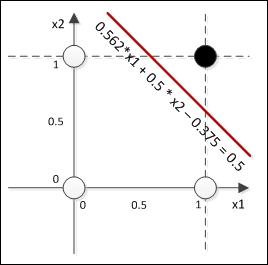
This boundary is a definition of all classifications given by the network. You can see that the boundary is linear, given that the function is linear. Thus, the perceptron network is really suitable for problems whose patterns are linearly separable.
Let's analyze the XOR case, whose chart can be seen in the following figure:

We see that in two dimensions, it is impossible to draw a line to separate the two patterns. What would happen if we tried to train a single-layer perceptron to learn this function? Suppose that we tried; let's see what happened through the following table:
|
Epoch |
x1 |
x2 |
w1 |
w2 |
b |
y |
t |
E |
Δw1 |
Δw2 |
Δb |
|---|---|---|---|---|---|---|---|---|---|---|---|
|
1 |
0 |
0 |
0,5 |
0,5 |
0,5 |
0,5 |
0 |
-0,5 |
0 |
0 |
-0,1 |
|
1 |
0 |
1 |
0,5 |
0,5 |
0,4 |
0,9 |
1 |
0,1 |
0 |
0,02 |
0,02 |
|
1 |
1 |
0 |
0,5 |
0,52 |
0,42 |
0,92 |
1 |
0,08 |
0,016 |
0 |
0,016 |
|
1 |
1 |
1 |
0,516 |
0,52 |
0,436 |
1,472 |
0 |
-1,472 |
-0,294 |
-0,294 |
-0,294 |
|
2 |
0 |
0 |
0,222 |
0,226 |
0,142 |
0,142 |
0 |
-0,142 |
0,000 |
0,000 |
-0,028 |
|
2 |
0 |
1 |
0,222 |
0,226 |
0,113 |
0,339 |
1 |
0,661 |
0,000 |
0,132 |
0,132 |
|
2 |
1 |
0 |
0,222 |
0,358 |
0,246 |
0,467 |
1 |
0,533 |
0,107 |
0,000 |
0,107 |
|
2 |
1 |
1 |
0,328 |
0,358 |
0,352 |
1,038 |
0 |
-1,038 |
-0,208 |
-0,208 |
-0,208 |
|
… |
… | ||||||||||
|
127 |
0 |
0 |
-0,250 |
-0,125 |
0,625 |
0,625 |
0 |
-0,625 |
0,000 |
0,000 |
-0,125 |
|
127 |
0 |
1 |
-0,250 |
-0,125 |
0,500 |
0,375 |
1 |
0,625 |
0,000 |
0,125 |
0,125 |
|
127 |
1 |
0 |
-0,250 |
0,000 |
0,625 |
0,375 |
1 |
0,625 |
0,125 |
0,000 |
0,125 |
|
127 |
1 |
1 |
-0,125 |
0,000 |
0,750 |
0,625 |
0 |
-0,625 |
-0,125 |
-0,125 |
-0,125 |
The perceptron just could not find any pair of weights that would drive the error below 0.625. This can be explained mathematically as we have already perceived from the chart that this function cannot be linearly separable in two dimensions. So, what if we add another dimension? Let's see the previous XOR chart in three dimensions:

In three dimensions, it is possible to draw a plane that would separate the patterns, provided that this additional dimension could properly transform the input data. Okay, but now, there is an additional problem: How can we derive this additional dimension since we have only two input variables? One obvious but "workaround" answer would be adding a third variable as a derivation from the two original ones. With this third variable a (derivation), our neural network would probably get the following shape:
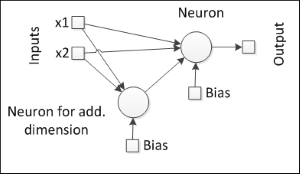
Okay, now, the perceptron has three inputs, one of them being a composition of the other two. This also leads to a new question: How should this composition be processed? We can see that this component can act as a neuron, thereby giving the neural network a nested architecture. If so, there would be another new question: How would the weights of this new neuron be trained, since the error is on the output neuron?