
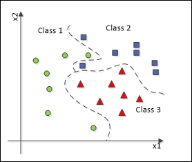
We've covered that neural networks can work as data classifiers by establishing decision boundaries onto data in the hyperspace. Such a boundary can be linear in the case of perceptrons or nonlinear in the case of other neural architectures such as MLPs, Kohonen, or Adaline. The linear case is based on linear regression, on which the classification boundary is literally a line, as shown in the preceding figure. If the scatter chart of the data looks like that shown in the following figure, then a nonlinear classification boundary is needed.
Neural networks are in fact a great nonlinear classifier, and this is achieved by the usage of nonlinear activation functions. One nonlinear function that actually works well for nonlinear classification is the sigmoid function, and the procedure for classification using this function is called logistic regression.
This function returns values bounded between 0 and 1. In this function, the α parameter denotes how hard the transition from 0 to 1 occurs. The following chart shows the difference:

Note that the larger the value of the α parameter is, the more the logistic function takes a shape of a hard-limiting threshold function, also known as a step function.
Classification problems usually deal with a case of multiple classes, where each class is assigned a label. However, a binary classification schema is applied in neural networks. This is because a neural network with a logistic function at the output layer can produce only values between 0 and 1, meaning that it assigns (1) or not (0) to some classes.
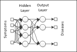
Nevertheless, there is one approach for multiple classes using binary functions. Consider that every class is represented by an output neuron, and whenever this output neuron fires, the neuron's corresponding class is applied on the input data record. So, let's suppose a network to classify diseases; each neuron output represents a disease to be applied to some symptom:
There is no perfect classifier algorithm; all of them are subjected to errors and biases. However, it is expected that a classification algorithm can correctly classify 70% to 90% of the records.
A confusion matrix shows how many of a given class's records were correctly classified and therefore how many were wrongly classified. The following table depicts what a confusion matrix may look like:
|
Actual class |
Inferred class |
Total | ||||||
|---|---|---|---|---|---|---|---|---|
|
A |
B |
C |
D |
E |
F |
G | ||
|
A |
92% |
1% |
0% |
4% |
0% |
1% |
2% |
100% |
|
B |
0% |
83% |
5% |
6% |
2% |
3% |
1% |
100% |
|
C |
1% |
3% |
85% |
0% |
2% |
5% |
4% |
100% |
|
D |
0% |
3% |
0% |
92% |
2% |
1% |
1% |
100% |
|
E |
0% |
10% |
2% |
1% |
78% |
1% |
8% |
100% |
|
F |
22% |
2% |
2% |
3% |
3% |
65% |
3% |
100% |
|
G |
9% |
6% |
0% |
16% |
0% |
3% |
66% |
100% |
Note that the main diagonal is expected to have higher values, as the classification algorithm will always try to extract meaningful information from the input dataset. The sum of all rows must be equal to 100% because all elements of a given class are to be classified in one of the available classes. However, note that some classes may receive more classifications than expected.
The more a confusion matrix looks like an identity matrix, the better the classification algorithm will be.
When the classification is binary, the confusion matrix is found to be a simple 2 x 2 matrix, and therefore, its positions are specially named:
|
Actual Class |
Inferred Class | |
|---|---|---|
|
Positive (1) |
Negative (0) | |
|
Positive (1) |
True Positive |
False Negative |
|
Negative (0) |
False Positive |
True Negative |
In disease diagnosis, which is the subject of this chapter, the concept of a binary confusion matrix is applied in the sense that a false diagnosis may be either a false positive or a false negative. The rate of false results can be measured by using sensitivity and specificity indexes.
Sensitivity denotes the true positive rate; it measures how many of the records are correctly classified positively.

Specificity in turn represents the true negative rate; it indicates the proportion of negative record identification.

High values of both sensitivity and specificity are desired; however, depending on the application field, sensitivity may carry more meaning.