17. Using SSDs to Solve I/O Bottlenecks

For most of the history of the Oracle relational database management system (RDBMS), the primary goal of performance tuning has been to avoid I/O at all cost. I/O to magnetic disk devices has always been many orders of magnitude slower than memory or CPU access, and the situation has only grown worse as Moore’s law accelerated the performance of CPU and memory while leaving mechanical disk performance behind. Solid-state drive (SSD) represents a revolutionary technology that provides a quantum leap in disk performance.

In recent years, SSD technology has shifted from an expensive luxury to a mainstream technology that has a place in almost every performance-critical Oracle database. Replacing all magnetic disk with SSD is sometimes infeasible because of the economics of increasingly large databases. Therefore, it becomes a new and critical requirement of the Oracle performance practitioner to understand the physics of solid-state devices and to employ them selectively to get the best return on investment.

To understand how flash technology contributes to Oracle performance and how best to exploit that technology, this chapter starts by comparing the performance and economics of flash and spinning disk technology. We then discuss how SSD can be deployed in Oracle databases to improve performance and solve I/O bottlenecks.

Moore’s law—first articulated by Intel founder Gordon Moore—observes that transistor density on a computer microchip doubles every 18 to 24 months. In its broadest interpretation, Moore’s law reflects the exponential growth that is commonly observed in almost all electronic components: improving CPU speed, RAM, and disk storage capacity.

While this exponential growth is observed in almost all electronic aspects of computing, including hard disk densities, it does not apply to mechanical technologies such as those underlying magnetic disk I/O. For instance, had Moore’s law been in effect for the rotational speed of disk devices, disks today would be rotating about 100 million times faster than in the early 1960s—in fact, they are rotating only eight times faster.

So while the other key components of computer performance have been advancing exponentially, magnetic disk drives have been improving only incrementally. There have been some significant technical innovations—Perpendicular Magnetic Recording, for instance—but these in general have led to improved capacity and reliability rather than speed. Consequently, disk drives are slower today (when compared to other components or even their own storage capacity) than in the past. As a result, disk I/O has been increasingly limiting the performance of database systems, and the practice of database performance tuning has largely become a process of avoiding disk I/O whenever possible.

In contrast to a magnetic disk, SSDs contain no moving parts and provide tremendously lower I/O latencies. Commercial SSDs are currently implemented using either double-data rate (DDR) RAM—effectively a battery-backed RAM device—or NAND flash. NAND flash is an inherently nonvolatile storage medium and almost completely dominates today’s SSD market.

Figure 17.3 illustrates the two competing trends: while the cost of I/O decreases with solid-state technology, the cost per terabyte increases. Various flavors of SSD (PCIe SATA and MLC/SLC) offer different price and performance characteristics compared to the various categories of magnetic disks (15 K vs. 7 K RPM). The SSD devices that offer good economies of I/O offer poorer economies for mass storage. Of course, the cost per gigabyte for SSD is dropping rapidly, but no faster than the falling cost of magnetic disks or the growth in database storage demand, especially in the era of Big Data.

Since most databases include both hot and cold data—small amounts of frequently accessed data as well as large amounts of idle data—most databases experience the best economic benefit by combining both solid-state and traditional magnetic disk technologies.

Oracle has implicitly acknowledged this in the architecture of the Exadata Database Machine, which combines both magnetic disks and flash disks to provide the optimal balance between storage economics and performance. If Exadata contained only magnetic disks, it could not provide superior online transaction processing (OLTP) performance; if it contained only SSD, it could not offer compelling economical storage for large databases.

The performance differences between SSDs and magnetic disks involve more than simply a reduction in read latency. Just as the fundamental architecture of magnetic disks favors certain I/O operations, the architecture of SSDs favors specific and different types of I/O. Understanding how an SSD handles the different types of operations helps us make the best decisions when choosing configuration options.

Until recently, MLC SSDs contained only 2 bits of information per cell. However, triple-level cache (TLC) SSDs are now becoming available: these are MLC devices that can store 3 bits of information, and in theory, higher-density MLCs may appear in the future. However, increasing the number of bits in each cell reduces the longevity and performance of the cell.

Cells are arranged in pages, typically 4 K or 8 K in size, and pages are arranged in blocks of between 128 K and 1 M, as shown in Figure 17.4.

Write I/O has another consequence in flash SSDs: after a certain number of writes, a cell may become unusable. This write endurance limit differs among drives but is typically between 10,000 cycles for a low-end MLC device and up to 1,000,000 cycles for a high-end SLC device. SSDs will generally fail safe when a cell becomes unwritable, marking the page as bad and moving the data to a new page.

Erase operations are avoided through the use of free lists and garbage collection. During an update, the SSD marks the block to be modified as invalid and copies the updated contents to an empty block, retrieved from a free list. Later, garbage collection routines recover the invalid block, placing it on a free list for subsequent operations. Some SSDs maintain storage above the advertised capacity of the drive to ensure that the free list does not run out of empty blocks for this purpose. This is known as overprovisioning.

Figure 17.6 illustrates a simplified SSD update algorithm. To avoid a time-consuming ERASE operation, the SSD controller marks a block to be updated as invalid (1), then takes an empty block from the free list (2) and writes the new data to that block (3). Later on, when the disk is idle, the invalid blocks are garbage collected by erasing the invalidated block.

Wear leveling is the algorithm that ensures that no particular block is subjected to a disproportionate number of writes. It may involve moving the contents of hot blocks to blocks from the free list and eventually marking overused blocks as unusable.

Wear leveling and garbage collection algorithms in the disk controller are what separates the men from the boys in SSDs. Without effective wear leveling and garbage collection, we would expect SSD drives to exhibit performance degradation and a reduced effective life. With the sophisticated algorithms employed by major SSD vendors, these issues are rarely significant.

However, the implications of garbage collection and wear leveling do influence what we expect from a database system that utilizes flash SSDs. Sustained heavy sequential write I/O or write operations that concentrate on a small number of hot pages may not allow the garbage collection and wear leveling algorithms time to clean up invalid pages or distribute hot pages between operations. As a result, SSDs subject to these sorts of workloads may exhibit performance or storage capacity degradation. This may influence decisions around the use of flash SSD for sequential write–intensive workloads such as those involved in redo log operations.

SATA SSDs are convenient because they can be attached wherever a traditional magnetic SATA disk is found. Unfortunately, the SATA interface was designed for magnetic disks, which have latencies in the order of milliseconds—thousands of microseconds. When a flash SSD, which has latencies in the order of microseconds, uses a SATA interface, the overhead of SATA becomes significant and may account for as much as two-thirds of the total read latency.

The PCIe interface was designed for extremely low-latency devices such as graphics adaptors, and allows these devices to interact directly with the computer’s processor bus. Consequently, PCIe SSD devices have much lower latencies than SATA SSD—read latencies in the order of 25 microseconds versus perhaps 75 microseconds for a typical SATA SSD.

Storage arrays are available that include PCIe- or SATA-based SSDs. These arrays may be composed exclusively of SSDs or may combine SSDs and magnetic disks in a hybrid array.

However, if you have a database server that has access to both magnetic disk and SSD, then your configuration may be more complex. You may choose to use SSD for selected tablespaces, segments, or in some cases as part of the Oracle Database Flash Cache.

The DBFC serves as a secondary cache to the Oracle buffer cache. Oracle manages data blocks in the buffer cache using a modified least recently used (LRU) algorithm. Simplistically speaking, blocks age out of the buffer cache if they have not been accessed recently. When the DBFC is active, blocks that age out of the buffer cache are not discarded but are instead written by the database writer (DBWR) to the flash device. Should the blocks be required in the future, they can be accessed from the flash cache instead of from database files residing on slower magnetic disk.

When a session wants to access an individual block of data from a table or index, it first looks for that block in the buffer cache. Oracle implements a complex algorithm to identify which blocks should be kept in memory. From a simplistic point of view, the longer it has been since the block was accessed, the more likely it is to be removed from the cache to make room for other blocks. This modified LRU algorithm is implemented by the LRU list—if a block is accessed, it may be moved up the list (metaphorically speaking). If blocks are not accessed, they may move down the list and eventually be aged out of the buffer cache.

When a data manipulation language (DML) statement modifies the contents of a block, the changes are made to a copy of the block in memory. The changed “dirty” buffer will not immediately be written to disk. The DBWR background process will write the dirty buffers out to database files at a later time. This deferred writing of changed blocks is generically known as a lazy write, and the principle is used by most databases.

Dirty (modified) buffers cannot be overwritten until the DBWR has written them to disk. If a session cannot find a clean buffer after scanning through the buffer cache, then it signals the DBWR to write modified buffers to disk and experiences a free buffer wait. By default, the session will scan 40 percent of the buffer cache before signaling the DBWR.

Free buffer waits are a commonly encountered form of buffer cache contention. They often occur when database read bandwidth exceeds write bandwidth—sessions attempt to load blocks into the buffer cache faster than they can be flushed to disk. Figure 17.7 illustrates the phenomenon.

The DBFC serves as a secondary cache to the Oracle buffer cache. When the flash cache is present, blocks that age out of the buffer cache are not discarded; they are instead written to the flash cache. Should the blocks be required in the future, they can be read from the flash cache instead of from database files residing on (presumably) slower magnetic disks.

Blocks are written to the flash cache by the DBWR process, which is normally responsible for writing modified blocks to datafiles. However, the DBWR maintains the flash cache as a secondary priority to its primary responsibility of writing out modified blocks to disk. Should the DBWR be busy with datafile writes, it will bypass flash cache maintenance. This “willful neglect” is designed to ensure that the maintenance of the flash cache does not inadvertently cause free buffer wait contention, which occurs when the DBWR cannot flush dirty buffers from the cache to disk in a timely manner.

Figure 17.8 shows the Oracle DBFC architecture. An Oracle server process reads blocks from the database files and stores them in the buffer cache (1). Subsequent reads can obtain the data buffers from the buffer cache without having to access the database file (2). When the block ages out of the buffer cache, the DBWR will load those blocks into the flash cache (3), but only if it does not interfere with writing modified blocks to disk (5). Subsequent reads may now find a block either in the flash cache (4) or the buffer cache (2).

The DB_FLASH_CACHE_FILE parameter may reference a file location on an SSD-backed file system or to an ASM disk group. In either case, Oracle will not necessarily validate that the location is SSD backed, so be careful to ensure that the locations are in fact located on a SSD device.

Following is an example of creating a DBFC on a file system. Note that the database must be restarted before the parameters take effect.

Click here to view code image

SQL> ALTER SYSTEM SET db_flash_cache_size=1024M SCOPE=SPFILE;
System altered.

SQL> ALTER SYSTEM SET
    db_flash_cache_file='/ssdfs/ora/dbfc/g11g_dbfc1.dbf'
    SCOPE=SPFILE;
System altered.

SQL> shutdown immediate
SQL> startup
ORACLE instance started.
SQL> show parameter flash_cache
NAME                 TYPE        VALUE
-------------------- ----------- ------------------------------
db_flash_cache_file  string      /ssdfs/ora/dbfc/g11g_dbfc1.dbf
db_flash_cache_size  big integer 1G

Setting the DB_FLASH_CACHE_SIZE parameter to 0 on a running database disables the flash cache.

You may encounter error ORA-00439 “feature not enabled: Server Flash Cache” when starting the database after configuring the flash cache. This is expected if the operating system is not an Oracle operating system (e.g., neither Solaris nor OEL) but can also occur due to bugs in early versions of Oracle 11g and 12g running on OEL 6—see MOS Note 1550735.1, “Database startup failing with ORA-00439 after enabling flash cache.”

NONE: Blocks will not be cached.

DEFAULT: Blocks will be cached at the normal priority.

KEEP: Blocks will be cached at high priority and will not be evicted from the cache unless there are no default blocks available.

The DBFC is mostly effective during indexed reads—because full table scans are likely to employ direct path reads, bypassing the buffer cache. Therefore, it is likely that you will want to apply the FLASH_CACHE clause to indexes as well as tables, as in the following example:

Click here to view code image

SQL> ALTER TABLE sales_fc_none STORAGE (FLASH_CACHE NONE);
Table altered.

SQL> ALTER INDEX sales_fc_pk STORAGE (FLASH_CACHE NONE);
Index altered.

SQL> ALTER TABLE sales_fc_default STORAGE (FLASH_CACHE DEFAULT);
Table altered.

SQL> ALTER INDEX sales_fc_default_pk STORAGE (FLASH_CACHE DEFAULT);
Index altered.

SQL> ALTER TABLE sales_fc_keep STORAGE (FLASH_CACHE KEEP);
Table altered.

SQL> ALTER INDEX sales_fc_keep_pk STORAGE (FLASH_CACHE KEEP);
Index altered.

Listing 17.1 DBFC SYSSTAT Counters (flash_insert_stats.sql)

Click here to view code image

---

SQL> WITH stats AS (SELECT  /*+ materialize */
  2                          name, VALUE
  3                   FROM   v$sysstat
  4                  WHERE   name LIKE 'flash cache%')
  5  SELECT name, VALUE,
  6         ROUND (VALUE * 100 / tot_inserts, 2) pct_of_inserts
  7    FROM (SELECT SUM (VALUE) tot_inserts
  8            FROM stats where name = 'flash cache inserts')
  9   CROSS JOIN  stats
 10   ORDER BY value DESC
 11  /

                                                              Pct of
NAME                                               VALUE     Inserts
---------------------------------------- --------------- -----------
flash cache insert skip: exists                3,224,749      551.26
flash cache insert skip: not useful            1,856,276      317.33
flash cache inserts                              584,974      100.00
flash cache eviction: aged out                   454,144       77.63
flash cache insert skip: DBWR overloaded          22,202        3.80
flash cache insert skip: modification              1,600         .27
flash cache eviction: invalidated                     22         .00
flash cache insert skip: not current                   1         .00
flash cache eviction: buffer pinned                    0         .00
flash cache insert skip: corrupt                       0         .00

---

These counters show how often blocks are inserted into the cache, how often they are evicted, and how often the DBWR is overloaded and so does not populate the cache.

Because the DBFC is an extension of the buffer cache, we can see the contents of the cache in the V$BH view. DBFC contents show up with a status of flashcur or flashcr. Listing 17.2 presents a query that displays the segments whose blocks are cached in buffer cache and/or DBFC.

Listing 17.2 DBFC Contents (flashContents.sql)

Click here to view code image

---

SQL>   SELECT   owner || '.' || object_name object,
  2       SUM (CASE WHEN b.status LIKE 'flash%' THEN 1 END) flash_blocks,
  3       SUM (CASE WHEN b.status LIKE 'flash%' THEN 0 else 1 END) cache_blocks,
  4       count(*) total_blocks
  5      FROM       v$bh b
  6             JOIN
  7                 dba_objects
  8             ON (objd = object_id)
  9  GROUP BY   owner, object_name
 10  order by 4 desc ;

                                   DBFC Buf Cache Tot Cached
Object Name                      Blocks    Blocks     Blocks
------------------------------ -------- --------- ----------
OPSG.SALES_FC_KEEP               70,450     1,325     71,775
OPSG.SALES_FC_KEEP_PK            34,155     2,325     36,480
OPSG.SALES_FC_DEFAULT            13,721       969     14,690
OPSG.SALES_FC_DEFAULT_PK         12,032     1,939     13,971
OPSG.SALES_FC_PK                            3,394      3,394
OPSG.SALES_FC_NONE                          2,305      2,305

---

Because a read from the flash cache is always a read that would otherwise have had to go to disk, it is possible to calculate how much time is saved by the flash cache. We do this by counting the number of flash cache reads and using the average flash cache latency together with the normal disk latency to calculate the amount of I/O time saved. Listing 17.3 shows the results. In general, if your database would benefit from a larger buffer cache, then it will almost certainly benefit from a DBFC.

Listing 17.3 DBFC Time Saved (flash_time_savings.sql)

Click here to view code image

---

SQL> WITH wait_table
  2          AS (SELECT   SUM (total_waits) total_waits,
  3                       SUM (time_waited_micro) total_time,
  4                       MAX(CASE event
  5                               WHEN 'db file sequential read'
  6                               THEN time_waited_micro / total_waits
  7                           END) avg_db_file_micro,
  8                       MAX(CASE event
  9                               WHEN 'db flash cache single block physical read'
 10                               THEN time_waited_micro / total_waits
 11                           END) avg_db_flash_micro,
 12                       SUM(CASE event
 13                               WHEN 'db flash cache single block physical read'
 14                               THEN total_waits
 15                           END) flash_waits
 16                FROM   v$system_event
 17               WHERE   event IN ('db file sequential read',
 18                                 'db flash cache single block physical read'))
 19  SELECT      total_waits,flash_waits,
 20           ROUND (avg_db_file_micro) avg_disk_time,
 21           ROUND (avg_db_flash_micro) avg_flash_time,
 22           total_time,
 23           ROUND(flash_waits *
 24                  (avg_db_file_micro - avg_db_flash_micro)) time_saved,
 25           ROUND(flash_waits *
 26                 (avg_db_file_micro - avg_db_flash_micro) * 100
 27                / (total_waits* avg_db_file_micro),2) pct_io_time_saved
 28    FROM      wait_table
 29   /

                      Flash Cache Avg Disk Avg DBFC           Total Time
     Total Waits            Waits  time us  time us                   us
---------------- ---------------- -------- -------- --------------------
          Time saved  Pct of IO
                  us Time saved
-------------------- ----------
       2,817,955        1,555,408    1,785       90        2,393,741,738
       2,636,254,812      52.41

---

The entire database might be deployed on SSD. For smaller databases, this may be the simplest option. However, this option is often economically impractical for large databases.

Selected datafiles, tables, indexes, or partitions could be located on SSD. This requires substantial planning and administration but is likely to be very effective if the correct segments are selected.

For databases that are of a compatible version and operating system type, the Oracle DBFC could be used. This option is simple to implement and can be very effective for read-intensive, index-based workloads.

The temporary tablespace could be relocated to SSD storage, accelerating the performance of temporary segment I/O, as occurs with disk sort or hashing operations.

Redo logs are inherently write intensive and have been suggested as candidates for SSD storage. However, as we shall see, the nature of redo log I/O is not a perfect fit for SSD.

In order to assess the likely performance benefits for each of the deployment options, the following sections provide simple performance tests that measure the performance of each configuration under appropriate workloads.

Using the DBFC resulted in a significant boost in performance—a reduction of 74 percent in elapsed time—whereas hosting the entire table (and its index) on SSD resulted in a 95 percent reduction.

Of course, you might expect DBFC performance to lag behind that of direct SSD, as the DBFC requires that the block be read from magnetic disk at least once. However, the DBFC does not require that there be sufficient SSD to store the entire segment, so it will be a more practical option in some circumstances.

The performance advantage of SSD is somewhat diminished when writes are involved, particularly for the DBFC. However, the performance advantages were still substantial: 69 percent reduction in elapsed time for the DBFC and 91 percent reduction when directly mounting the segment on SSD.

Not surprisingly, placing the table on SSD resulted in a dramatic improvement in full table scan performance. However, using the DBFC did not result in any measurable performance improvement. From Oracle 11g onward, full table scans typically bypass the buffer cache: the Oracle process reads directly from disk and does not place the blocks thus read in the buffer cache. Since the Database Flash Case is populated from the buffer cache, full table scans cannot normally benefit from the DBFC.

Figure 17.12 illustrates this approach using Dell FluidCache as an example. The cache interposes itself between some traditional storage devices and an SSD device. The merged device is presented to the operating system as a single LUN, with the SSD being used to cache frequently accessed data.

The advantage in an Oracle context is that this form of cache makes no differentiation between direct path I/O and any other I/O. Therefore, this form of caching is capable of accelerating full table scans in a way that the DBFC cannot.

Figure 17.13 illustrates this phenomenon using Fusion-io directCache. When the cache is enabled, second and subsequent scans of a table show acceleration.

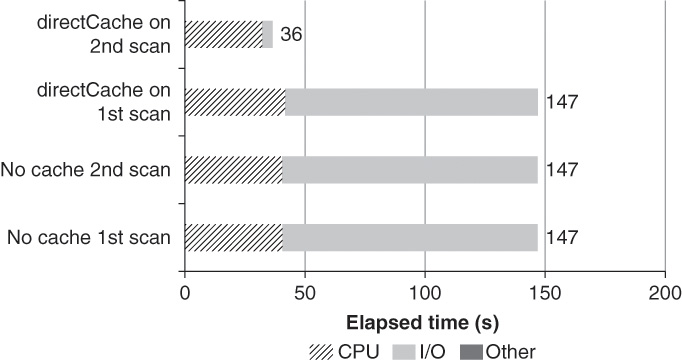
Another advantage of these technologies is that they can be used on any operating system, while the DBFC can be used only on Oracle operating systems.

As memory becomes constrained, temporary segment I/O requirements for the operation come to dominate performance and rise sharply as the number of temporary segment passes increase.

When the temporary tablespace is placed on SSD, a completely different performance profile emerges, as shown in Figure 17.15. While the overhead of single-pass sorts are significantly improved, the overhead of multipass disk sorts is drastically reduced. The more temporary segment passes are involved, the greater is the improvement.

Since redo log I/O is so often a performance bottleneck, many have suggested locating the redo logs on SSD for performance optimization. However, the nature of redo log I/O is significantly different from that of datafile I/O; redo log I/O consists almost entirely of sequential write operations without any seek time for which magnetic disk is well suited, since write throughput is limited only by the rotation of the magnetic disk. In contrast, the sequential write–intensive workload is a worst-case scenario for SSD, since as we have seen, write I/O is far slower than read I/O for SSDs.

Figure 17.16 shows how placing of redo logs on an SSD device in the case of a redo I/O–constrained workload resulted in no measurable improvement in performance. In this case, the SAS drive was able to support a write rate equal to that of the SSD device.

In more than 15 years of writing on Oracle performance, nothing I’ve ever presented has caused so much controversy as the results I’ve presented on redo log performance using SSD. Many people have argued that SSD is a good foundation for redo logs. However, to date, no one has presented data that clearly contradicts the essential point shown in Figure 17.16. Although it is definitely possible to get a slight improvement in performance with very high-end dedicated SSD, we never see the huge improvements that we get with other workloads, such as for index reads or temporary tablespaces. And these results do match with theoretical expectations—we know that sequential write operations are the worst possible type of I/O for SSD and the best possible type of I/O for magnetic disk.

Oracle DBAs must balance two competing demands:

Increasing data volumes (Big Data) require solutions that provide economical storage for masses of data, which essentially requires systems that incorporate magnetic disk.

Increasing transaction rates and exponential increases in CPU capacity require solutions that provide economical provision of I/O operations per second (IOPS) and minimize latency. This is the province of SSD and in-memory solutions.

For many or even most databases, the only way to balance both of these trends is to “tier” various forms of storage, including RAM, SSD, and magnetic disk. The Oracle database provides a variety of mechanisms that allow you to move data between the tiers to balance IOPS and storage costs and maximize performance. Following are the key capabilities that you should consider:

Partitioning: This technique allows an object (table or index) to be stored across various forms of storage and allows data to be moved online from one storage medium to another.

Compression: Compression can be used to reduce the storage footprint (but may increase the retrieval time).

Oracle 12 Automatic Database Optimizer (ADO): ADO allows policy-based compression of data based on activity or movement of segments to alternative storage based on free space.

Oracle partitioning allows a table’s data to be stored in multiple segments (i.e., partitions), and those partitions can be stored in separate tablespaces. It is therefore the cornerstone of any database storage tiering solution.

A complete discussion of all of the Oracle partitioning capabilities is beyond the scope of this chapter. However, let’s consider a scheme that could work to spread the contents of a table across two tiers of storage. The hot tier is stored on a flash-based tablespace, while the cold tier is stored on an HDD-based tablespace.

Interval partitioning allows us to nominate a default partition for new data while selecting specific storage for older data.

Listing 17.4 provides an example of an interval partitioned table. New data inserted into this table is stored in partitions on the SSD_TS tablespace, while data older than July 1, 2013, is stored on the SAS_TS tablespace.

Listing 17.4 Interval Partitioned Table

Click here to view code image

---

CREATE TABLE ssd_partition_demo
(
   id            NUMBER PRIMARY KEY,
   category      VARCHAR2 (1) NOT NULL,
   rating        VARCHAR2 (3) NOT NULL,
   insert_date   DATE NOT NULL
)
PARTITION BY RANGE (insert_date)
   INTERVAL ( NUMTOYMINTERVAL (1, 'month') )
    STORE IN (ssd_ts)
   (PARTITION cold_data VALUES LESS THAN
         (TO_DATE ('2013-07-01', 'SYYYY-MM-DD'))
         TABLESPACE sas_ts);

---

After some data has been loaded into the table, we can see that new data is stored on the SSD-based tablespace (SSD_TS), and older data is stored on the SAS based tablespace (SAS_TS):

Click here to view code image

SQL> l
  1  SELECT partition_name, high_value, tablespace_name
  2    FROM user_tab_partitions
  3*  WHERE table_name = 'SSD_PARTITION_DEMO'
SQL> /

PARTITION HIGH_VALUE                               TABLESPACE
--------- ---------------------------------------- ----------
COLD_DATA TO_DATE(' 2013-07-01 00:00:00', 'SYYYY-M SAS_TS
          M-DD HH24:MI:SS', 'NLS_CALENDAR=GREGORIA
SYS_P68   TO_DATE(' 2013-11-01 00:00:00', 'SYYYY-M SSD_TS
          M-DD HH24:MI:SS', 'NLS_CALENDAR=GREGORIA
SYS_P69   TO_DATE(' 2013-12-01 00:00:00', 'SYYYY-M SSD_TS
          M-DD HH24:MI:SS', 'NLS_CALENDAR=GREGORIA
SYS_P70   TO_DATE(' 2013-10-01 00:00:00', 'SYYYY-M SSD_TS
          M-DD HH24:MI:SS', 'NLS_CALENDAR=GREGORIA
SYS_P71   TO_DATE(' 2013-09-01 00:00:00', 'SYYYY-M SSD_TS
          M-DD HH24:MI:SS', 'NLS_CALENDAR=GREGORIA
SYS_P72   TO_DATE(' 2013-08-01 00:00:00', 'SYYYY-M SSD_TS
          M-DD HH24:MI:SS', 'NLS_CALENDAR=GREGORIA
SYS_P73   TO_DATE(' 2014-01-01 00:00:00', 'SYYYY-M SSD_TS
          M-DD HH24:MI:SS', 'NLS_CALENDAR=GREGORIA
SYS_P74   TO_DATE(' 2014-02-01 00:00:00', 'SYYYY-M SSD_TS
          M-DD HH24:MI:SS', 'NLS_CALENDAR=GREGORIA

This configuration is initially suitable, but of course as data ages, we would want to move less frequently accessed data from the SSD tablespace to a SAS-based tablespace. To do so, we issue an ALTER TABLE MOVE PARITION statement.

For instance, the PL/SQL in Listing 17.5 moves all partitions with a HIGH_VALUE of more than 90 days ago from the SSD_TS tablespace to the SAS_TS tablespace.

Listing 17.5 PL/SQL to Move Old Partitions from SSD to SAS Tablespace

Click here to view code image

---

DECLARE
   num_not_date         EXCEPTION;
   PRAGMA EXCEPTION_INIT (NUM_NOT_DATE, -932);
   invalid_identifier   EXCEPTION;
   PRAGMA EXCEPTION_INIT (invalid_identifier, -904);

   l_highdate           DATE;
BEGIN
   FOR r IN (SELECT table_name,
                    partition_name,
                    high_value
               FROM user_tab_partitions
              WHERE tablespace_name <> 'SSD_TS')
   LOOP
      BEGIN
         -- pull the highvalue out as a date
         EXECUTE IMMEDIATE 'SELECT ' || r.high_value || ' from dual'
            INTO l_highdate;

         IF l_highdate < SYSDATE - 90
         THEN
            EXECUTE IMMEDIATE
                  'alter table '
               || r.table_name
               || ' move partition "'
               || r.partition_name
               || '" tablespace sas_ts';
         END IF;
      EXCEPTION
         WHEN num_not_date OR invalid_identifier   -- max_value not a date
         THEN
            NULL;
      END;
   END LOOP;
END;

---

In Oracle Database 11g, this operation blocks DML on each partition during the move (or fails with error ORA-00054 if the partition can’t be locked). In Oracle Database 12c, you may specify the ONLINE clause to allow transactions on the affected partition to continue. After the move, local indexes corresponding to the moved partition and all global indexes are marked as unusable unless you specify the UPDATE INDEXES or UPDATE GLOBAL INDEXES clause.

The Oracle Database 12c syntax for moving partitions online is simple and effective, whereas in Oracle Database 11g, we can achieve the same result albeit in a more complex manner. Using the DBMS_REDEFINITION package, we can create an interim table in the target tablespace, synchronize all changes between that interim table and the original partition, and then exchange that interim table for the original partition.

Listing 17.6 provides an example of using DBMS_REDEFINITION. We create a distinct interim table INTERIM_PARTITION_STORAGE in the target tablespace SAS_TS, which is synchronized with the existing partition SYS_P86. When the FINISH_REDEF_TABLE method is invoked, all transactions that may have been applied to the existing partition SYS_P86 are guaranteed to have been applied to the interim table, and the table is exchanged with the partition concerned. The interim table, which is now mapped to the original partition segment, can now be removed.

Listing 17.6 Using DBMS_REDEFINITION to Move a Tablespace Online

Click here to view code image

---

-- Enable/ Check that table is eligible for redefinition
BEGIN
  DBMS_REDEFINITION.CAN_REDEF_TABLE(
   uname        => USER,
   tname        => 'SSD_PARTITION_DEMO',
   options_flag => DBMS_REDEFINITION.CONS_USE_ROWID,
   part_name    => 'SYS_P86');
END;
/
-- Create interim table in the tablespace where we want to move to
CREATE TABLE interim_partition_storage TABLESPACE sas_ts
AS SELECT * FROM ssd_partition_demo PARTITION (sys_p86) WHERE ROWNUM <1;

-- Begin redefinition
 BEGIN
  DBMS_REDEFINITION.START_REDEF_TABLE(
   uname        => USER,
   orig_table   => 'SSD_PARTITION_DEMO',
   int_table    => 'INTERIM_PARTITION_STORAGE',
   col_mapping  => NULL,
   options_flag => DBMS_REDEFINITION.CONS_USE_ROWID,
   part_name    => 'SYS_P86');
END;
/
-- If there are any local indexes create them here
-- Synchronize
BEGIN
  DBMS_REDEFINITION.SYNC_INTERIM_TABLE(
   uname      => USER,
   orig_table => 'SSD_PARTITION_DEMO',
   int_table  => 'INTERIM_PARTITION_STORAGE',
   part_name  => 'SYS_P86');
END;
/

-- Finalize the redefinition (exchange partitions)
BEGIN
  DBMS_REDEFINITION.FINISH_REDEF_TABLE(
   uname      => USER,
   orig_table => 'SSD_PARTITION_DEMO',
   int_table  => 'INTERIM_PARTITION_STORAGE',
   part_name  => 'SYS_P86');
END;
/

---

Using DBMS_REDEFINITION is cumbersome, but generally it is the best approach in Oracle Database 11g when you expect that the partition being moved may be subject to ongoing transactions. In Oracle Database 12c, using the ONLINE clause of MOVE PARTITION is far easier.

Oracle Exadata systems combine SSD and magnetic disk to provide a balance between economies of storage and high performance. In an Exadata system, flash SSD is contained in the storage cells only. There is no SSD configured within the compute nodes.

Each storage cell contains four PCIe flash SSD drives. The exact configuration depends on the Exadata version. On an X4 system, each cell contains four 800 GB Sun F80 MLC PCI flash cards. That’s 3.2 TB of flash per cell and a total of 44.8 TB of flash for a full Exadata rack!

The default configuration for Exadata flash configures all flash storage as Exadata Smart Flash Cache (ESFC). The Exadata Smart Flash Cache is analogous to the Oracle DBFC but has a significantly different architecture. The primary purpose of the Exadata Smart Flash Cache is to accelerate read I/O for database files. This is done by configuring flash as a cache over the grid disks that service datafile read I/O. Figure 17.17 illustrates the mapping on flash disks to Exadata Smart Flash Cache.

For suitable OLTP-style workloads, the Exadata Smart Flash Cache provides a fourfold or even better improvement in throughput. By default, the Exadata Smart Flash Cache does not accelerate smart scans or full table scans. You can enable caching of full and smart scans by setting CELL_FLASH_CACHE KEEP in the segment STORAGE clause. This clause, if set to NONE, can completely disable caching for a segment. Although the KEEP setting can accelerate scan performance, it does involve some overhead as the cache is loaded and might even degrade overall cache efficiency—so apply it judiciously.

From Oracle Database 11.2.2.4 onward, Exadata Smart Flash Logging allows the flash cache to participate in redo log write operations also. As shown in Figure 17.18, during a redo log write, the Exadata storage server will write to the flash and grid disks simultaneously and return control to the log writer when the first of the two devices completes. This helps alleviate the occasional very high redo write “outliers.”

From Oracle Database 11.2.3.2.1 onward, the Exadata Smart Flash Cache can become a write-back cache, allowing it to satisfy write requests as well as read requests. In normal circumstances, Oracle sessions do not wait on database writes, but in the event that free buffer waits are experienced as a result of read bandwidth surpassing write bandwidth, the write-back cache can break the bottleneck and accelerate throughput.

Placing a table directly on flash storage will provide better performance than the Exadata Smart Flash Cache in most circumstances, since it would obviate the need for initial reads from SAS disk to populate the cache, and data will never age out of flash. The degree of improvement in performance will depend on the data access patterns and the size of the segment (or segments). Figure 17.20 shows the results of performance comparison for an OLTP workload with data on HDD only, on HDD with flash cache, and on SSD.

Smaller segments that are subject to infrequent scans will show the most benefit, since by default the Exadata Smart Flash Cache does not optimize scan I/O. Index reads will also benefit, though the benefit may be marginal when the hit rate in the Exadata Smart Flash Cache is very high.

Redo logs generate significant I/O and can be a transactional bottleneck. However, as we discussed earlier, the I/O patterns of redo activity—sequential write activity—favor spinning magnetic disk over flash SSD.

As we learned in this chapter, there are a variety of ways that we can use SSD in Oracle databases:

Place the entire database on flash—if we can afford it.

Use the Oracle DBFC to accelerate index read I/O. However, this is possible only if your database is running on an Oracle operating system—Oracle Linux or Solaris.

Place selected hot segments on a tablespace based on SSD.

Locate the temporary tablespace on SSD. This approach is attractive if temporary tablespace I/O dominates performance.

Place redo logs on SSD. However, both theory and observation suggest this solution provides the lowest return on SSD investment.