Chapter 3: Reporting Different Metrics Within a Column

Introduction

Example: Demographic and Baseline Characteristics Report

Goals for the Demographics and Baseline Characteristics Report

Key Steps

Source Data

ODS Style Template Used

Programs Used

Implementation

Obtain Population Counts for Column Headers and Denominators

Code for Obtaining Population Counts

Categorical Variables: Obtain Counts and Percentages

Code for Obtaining Categorical Counts and Percentages

Continuous Variables: Descriptive Data

Macro Code for Obtaining Descriptive Statistics

Create Final Table: Combine TABULATE and MEANS Results

Code for Combing the Results

Produce the Report via PROC REPORT

PROC REPORT Code

Chapter 3 Summary

Introduction

One reporting challenge arises when various data types need to be reported within a column. This is often the case in a Clinical Trials Demographics and Baseline Characteristics report, in which some of the raw data variables are categorical while others are continuous. The categories are reported as counts and percentages, while the continuous variables are summarized by a set of descriptive statistics such as the mean, median, standard deviation, and minimum and maximum values. In addition, the metrics require varying levels of precision and call for the summaries to line up visually by using indentation and/or decimal alignment.

Example: Demographic and Baseline Characteristics Report

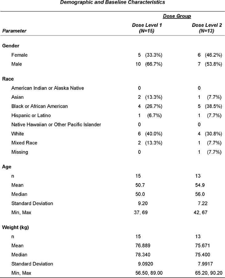
For this example, patients are randomly assigned to one of two treatment groups, each group having a corresponding planned dose level of Study Medication (Dose Level 1 versus Dose Level 2). Four demographic and baseline characteristics are reported for each treatment group. Gender and Race are categorical variables, while Age and Weight are continuous variables. Figure 3.1 displays the report to be produced in this chapter.

Figure 3.1 Chapter 3 Report

Goals for the Demographics and Baseline Characteristics Report

The goals for the Demographics and Baseline Characteristics report include:

 

• Reporting varying data types within a column, such as:

∘ Categorical data (Gender and Race) versus Continuous data (Age and Weight).

– Different metrics: counts and percentages for categorical data; n, mean, median, standard deviation, minimum and maximum for continuous variables.

• Application of desired precision with the help of macro variables.

∘ Percentages are reported to one decimal.

∘ Number of decimal places reported for continuous statistics depends on the specific variable and statistic being reported.

• Alignment of decimals and other alignment for the various metrics.

• For categorical variables, reporting all categories on the data collection form, even if there were no occurrences in the data.

Key Steps

The key steps taken to accomplish the goals include:

 

1. Obtaining the column N’s (population counts) for display in the report column headers.

2. Use of the TABULATE and MEANS procedures to obtain the needed metrics and output data sets.

3. Modifying the TABULATE and MEANS output data sets to arrive at the common structure needed for the final output.

∘ Applying rounding to numeric data

∘ Converting numeric data to character strings

∘ Deriving variables needed for a common data structure

∘ Transposing the data to get treatment groups across the top.

4. Concatenating PROC TABULATE and PROC MEANS output once the data sets have a common structure.

5. Using ODS and PROC REPORT to style the report.

Source Data

There is one source data set named Ch3Demo. Ch3Demo contains a patient’s demographic information, including the variables AGE, RACE, GENDER, and WEIGHTKG (weight in kilograms), each patient’s identification number (SUBJID), and the treatment group to which they were assigned (TRT).

Tables 3.1 and 3.2 display the variable information and partial data for the data set “Ch3Demo”.

Table 3.1 Ch3Demo Variable Information

#	Variable	Type	Len	Label
1	SUBJID	Char	8	Patient ID
2	TRT	Char	8	Treatment Group
3	RACE	Char	8	Race
4	GENDER	Char	8	Gender
5	WEIGHTKG	Num	8	Weight (kg)
6	AGE	Num	8	Age (years)

 

Table 3.2 Partial Ch3Demo Data

SUBJID	TRT	RACE	GENDER	WEIGHTKG	AGE
1	1	BA	M	80.00	44
3	1	WH	M	77.30	47
4	1	WH	M	82.40	50
5	1	WH	F	62.66	37
7	1	HL	M	68.60	48
8	1	MX	M	84.00	60
9	1	MX	M	88.60	55
10	1	WH	M	76.20	52

 

ODS Style Template Used

The report is produced in the Output Delivery System (ODS) Rich Text Format (RTF) destination. The Journal style template is used and specified prior to the PROC REPORT section in the statement

ods rtf style=journal file=“{PATHFILENAME}.rtf”;

Programs Used

One program, Ch3Demo.sas, is used to create the Demographics and Baseline Characteristics Report.

Implementation

The remainder of the chapter describes the steps taken to create the Demographics and Baseline Characteristics report.

PROC TABULATE is used to obtain the counts and percentages for GENDER and RACE.

PROC MEANS is used to obtain descriptive statistics for the continuous variables AGE and WEIGHTKG, including the mean, median, standard deviation, minimum and maximum values and the number of observations on which the statistics are based.

Because the TABULATE and MEANs output require slightly different processing, these sections are demonstrated separately.

Obtain Population Counts for Column Headers and Denominators

The population counts are obtained for each treatment (dose level) group. The count for each population is saved into its own macro variable for later reporting of the population count in each treatment group column header.

Key steps for obtaining population counts include:

 

• Getting Population Counts via PROC FREQ.

• Storing Treatment Group Population Counts in Macro Variables &POP1 and &POP2.

Code for Obtaining Population Counts

 

** Get Data;

data demo;

     set sasuser.ch3demo;

run;

** Get Population Counts via PROC FREQ;

proc freq data= demo noprint; ➊

   tables trt /out=pop;

run;

** Store Treatment Group Population Counts in Macro Variables;

data _null_;

   set pop;

   call symputx(“POP” || TRT, COUNT); ➋

run;

%put Population for trt1 = &pop1;

%put Population for trt2 = &pop2;

➊ A PROC FREQ is run to obtain the population counts for each treatment group.

➋ CALL SYMPUTX is used to pass the population counts for TRT=1 and TRT=2 into the macro variables, &POP1 and &POP2, respectively. The %PUT statements result in the log showing the following population counts:

Population for trt1 = 15

Population for trt2 = 13

Categorical Variables: Obtain Counts and Percentages

The key steps taken to prepare the categorical data for the final report include:

• Add PICTURE Format for Character Percent Alignment.

• Add formats to be used in PROC TABULATE.

• Use the TABULATE procedure to obtain the categorical variable counts and percentages for all categories specified in preloaded formats. Output the results to data sets.

• Create a character string that concatenates count and percent in the form n (xx.x). The percentages are rounded prior to being converted to character type.

• Derive variable VARNAME, needed for the final output structure.

• Transpose the TABULATE output data sets to get treatment groups across the top. SUBCAT, another variable needed for the final output structure, is obtained in this step.

Code for Obtaining Categorical Counts and Percentages

 

**   Create needed formats; ➊

proc format;

   **   Add PICTURE Format for Character Percentage Alignment;

   picture pctdec (round)

       0 – 1000 = “0009.9%)” (prefix=“(“)

       Other     = “ “;

   **   Add Formats to be preloaded in the TABULATE procedure;

   **   We will use PRELOADFMT to produce rows with zero observations;

   value $sex

       “F”  = “Female”

       “M” = “Male”;

  

   value $race

       “AI”   = “American Indian or Alaska Native”

       “AS”  = “Asian”

       “BA”  = “Black or African American”

       “WH”= “White”

       “HL”  = “Hispanic or Latino”

       “MX” = “Mixed Race”

       “NH” = “Native Hawaiian or Other Pacific Islander”

       “ “     = “Missing”;

run;

%MACRO TAB(tabvar=, indat=demo, fmt=, debug=N);

/** A Macro for Character Variables **/

/** Obtain Counts and Percentages **/ ➋

   proc tabulate data=&indat missing

                           out=m_&tabvar.1(drop=_type_ _page_ _table_);

       by trt;

       class &tabvar   / preloadfmt;

       table &tabvar, n*f=8. pctn / misstext=“0” printmiss;

       format &tabvar &fmt..;

   run;

   data m_&tabvar.2;

       length &tabvar varname $16 pctc $30;

       set m_&tabvar.1;

/** Create Character String for Count and Percentage **/ ❸

       if pctn_0=0 then pctc=“0”;

       else pctc = strip(put(n,3.)|| " " ||put(pctn_0,pctdec.));

/** Derive Variable Needed for Final Output Structure **/

       varname= upcase("&tabvar"); ➍

   run;

/** Transpose the TABULATE Data **/

   proc sort data=m_&tabvar.2 out=m_&tabvar.3;

       by varname &tabvar trt;

   run;

   proc transpose data=m_&tabvar.3

           out=m_&tabvar.4(drop=_NAME_ rename=(&tabvar=subcat))

           prefix=trt; ➎

       by varname &tabvar;

       id trt;

       var pctc;

   run;

/** Delete Unnecessary Data Sets After Debugging is Complete **/

   %if &debug=Y %then

       %do;

           proc sql;

               drop table m_&tabvar.1,

                                m_&tabvar.2,

                                m_&tabvar.3;

           quit;

       %end;

%MEND TAB;

%TAB(tabvar=gender, indat=demo, fmt=$sex,   debug=Y)

%TAB(tabvar=race   ,   indat=demo, fmt=$race, debug=Y)

➊ A picture format is created for standardizing the character percent format. The (ROUND) option is added to the picture statement so percentages will be rounded before a format is applied. The picture format specification

0 - 1000 =“0009.9%)” (prefix=“(“)

easily decimal aligns the percentages, adds a % sign, and surrounds the string in parentheses without leading and trailing blanks. The example below shows that the Race percentages are decimal aligned.

The $SEX and $RACE formats are created to pre-specify (preload) the desired categories to be shown in the TABULATE procedure output.

 

For each categorical variable (SEX and RACE in this example), the following steps are implemented via a macro call.

 

➋ PROC TABULATE is run and the counts and percentages are saved to an output dataset containing the name of the variable.

The guideline for this report is to display all possible categories shown on the data collection form even when there are no occurrences in the actual data. The following specifications in PROC TABULATE allow us to obtain the counts and percentages for all possible categories.

• The MISSING option in the PROC TABULATE statement includes an observation that contains a missing value for a class variable. Without the MISSING option, observations with missing values for class variables would not be included in the analysis.

• The PRELOADFMT in the CLASS statement, along with PRINTMISS in the TABLE statement, are used to display all possible combinations of formatted class variable values. This allows us to show when there are zero cases of a formatted value, for example, in our data set, the race=“American Indian or Alaskan Native” category does not occur.

• The format statement specifies the format to apply to each class variable.

• MISSTEXT=“0” specifies that the text “0” should be printed rather than the default period (“.”) to represent missing values.

❸ The character string PCTC is created. PCTC contains count and percentage in the form n (xx.x). The character percentage portion (xx.x) is created with the picture format pctdec. The string will be decimal aligned in the RTF output when the column style just=d is used.

➍ Because the individual TABULATE output data sets will be concatenated later on, the identification variable VARNAME is added to each output data set. Table 3.3 shows the PROC PRINT for RACE at this point in the process.

Table 3.3 TABULATE Data for RACE – Pre-Transpose

varname	TRT	race	N	PctN_0	pctc
RACE	1	Missing	.	0.0000	0
RACE	1	American Indian or Alaska Native	.	0.0000	0
RACE	1	Asian	2	13.3333	2 (13.3%)
RACE	1	Black or African American	4	26.6667	4 (26.7%)
RACE	1	Hispanic or Latino	1	6.6667	1 (6.7%)
RACE	1	Mixed Race	2	13.3333	2 (13.3%)
RACE	1	Native Hawaiian or Other Pacific Islander	.	0.0000	0
RACE	1	White	6	40.0000	6 (40.0%)
RACE	2	Missing	1	7.6923	1 (7.7%)
RACE	2	American Indian or Alaska Native	.	0.0000	0
RACE	2	Asian	1	7.6923	1 (7.7%)
RACE	2	Black or African American	5	38.4615	5 (38.5%)
RACE	2	Hispanic or Latino	1	7.6923	1 (7.7%)
RACE	2	Mixed Race	1	7.6923	1 (7.7%)
RACE	2	Native Hawaiian or Other Pacific Islander	.	0.0000	0
RACE	2	White	4	30.7692	4 (30.8%)

 

➎ The data are transposed so that the categorical variable is reported with Treatment Groups 1 and 2 across the top. The &tabvar variable (RACE in this case) is renamed to “SUBCAT”, one of the needed variables for the final output data structure. Table 3.4 shows the PROC PRINT for RACE, after the transpose.

Table 3.4 Transposed Data for RACE

varname	subcat	trt1	trt2
RACE	Missing	0	1 (7.7%)
RACE	American Indian or Alaska Native	0	0
RACE	Asian	2 (13.3%)	1 (7.7%)
RACE	Black or African American	4 (26.7%)	5 (38.5%)
RACE	Hispanic or Latino	1 (6.7%)	1 (7.7%)
RACE	Mixed Race	2 (13.3%)	1 (7.7%)
RACE	Native Hawaiian or Other Pacific Islander	0	0
RACE	White	6 (40.0%)	4 (30.8%)

The other category variables are run through the TAB macro as well to generate output that looks similar in structure to the RACE output.

Continuous Variables: Descriptive Data

The MEANS macro is used to generate the needed statistics via PROC MEANS and to perform additional processing that structures the MEANS data similarly to the TABULATE data.

The key steps taken to prepare the MEANS data for the final report include:

 

• Use of the MEANS procedure to obtain the continuous variable descriptives and output data sets.

• Round output data to the appropriate decimal places.

• Convert numeric metrics to character versions.

• Concatenate minimum and maximum values in the form min, max.

• Derive variable needed for the final output structure, VARNAME.

• Transpose the MEANS output data sets to get treatment groups across the top. SUBCAT, another variable needed for the final output structure, is obtained in this step.

Macro Code for Obtaining Descriptive Statistics

 

%MACRO MEANS(meanvar=,indata=demo,rawdec=,rnddec=,debug=N); ➊

   /** Use PROC MEANS to Obtain Continuous Variable Descriptives **/

   proc means data=&indata noprint;

       class trt;

       var &meanvar;

       output out=m_&meanvar.1(where=(_TYPE_ ne 0))

                           n=N p50=MED mean=MEAN stddev=SD min=MIN max=MAX; ➋

   run;

   data m_&meanvar.2;

       length varname $16 nc meanc medc sdc minmaxc $50;

       set m_&meanvar.1(drop=_TYPE_ _FREQ_);

   /** Round Mean, Median, and SD **/ ➌

       if mean ne . then mean = round(mean,.&rnddec);

       if med   ne . then med   = round(med ,.&rnddec);

       if sd      ne . then sd       = round(sd   ,.0&rnddec);

   /** Create Character Versions of Statistics **/ ➍

       meanc    = strip(put(mean,12.%eval(&rawdec+1)));

       medc      = strip(put(med ,12.%eval(&rawdec+1)));

       sdc         = strip(put(sd   ,12.%eval(&rawdec+2)));

       nc           = strip(put(n     ,12.));

       minc       = strip(put(min ,12.&rawdec));

       maxc      = strip(put(max ,12.&rawdec));

   /** Concatenate minimum and maximum values in the form min, max **/

       minmaxc = strip(minc) || ", " || strip(maxc); ➎

   /** Derive Variable Needed for Final Output Structure **/

       varname = upcase("&meanvar"); ➏

   run;

   /** Transpose the MEANS Data **/

   proc sort data=m_&meanvar.2 out=m_&meanvar.3;

       by varname trt;

   run;

   proc transpose data=m_&meanvar.3

       out=m_&meanvar.4

               prefix=trt name=subcat; ➐

       by varname;

       id trt;

       var nc meanc medc sdc minmaxc;

   run;

/** Delete Unnecessary Data Sets After Debugging is Complete **/

%if &debug=Y %then

       %do;

           proc sql;

               drop table m_&meanvar.1,

                                m_&meanvar.2,

                                m_&meanvar.3;

           quit;

       %end;

%MEND MEANS;

%MEANS(meanvar=AGE,              indata=demo,rawdec=0,RNDDEC=1,   debug=Y)

%MEANS(meanvar=WEIGHTKG,indata=demo,rawdec=2,RNDDEC=001,debug=Y)

➊ Macro parameters include:

Macro Variable	Description
&MEANVAR	the variable for which statistics are being obtained (e.g., AGE, WEIGHTKG)
&INDATA	the input dataset name
&RAWDEC	represents the maximum number of decimal places reported in the raw data for that variable
&RNDDEC	contains the needed precision for the round functions
&DEBUG	Specify if debugging is complete. If so, interim unneeded data sets will be deleted

 

➋ The needed PROC MEANS statistics are saved to an output dataset.

➌ Means, medians, and standard deviations are rounded using the ROUND function along with &RNDDEC to specify the rounding unit.

For this report, each variable’s means and medians are reported to one decimal place beyond the maximum amount of decimal places found in the raw data for that variable. Standard deviations are reported to two decimal places beyond the maximum amount of decimal places found in the raw data for that variable.

For AGE, the maximum number of decimal points in the raw data is 0, therefore &RAWDEC is set to 0 in the macro call. Setting &RNDEC to 1 in the macro call arrives at the correct rounding since MEAN and MED are rounded to “.&RNDDEC” and SD is rounded to “.0&RNDDEC”.

The rounding unit for AGE becomes the shaded portion of the following code upon macro resolution:

MPRINT(MEANS):     if mean ne . then mean = round(mean,.1);

MPRINT(MEANS):     if med   ne . then med   = round(med ,.1);

MPRINT(MEANS):     if sd      ne . then sd       = round(sd   ,.01);

➍ Character versions of each statistic are created using PUT functions and the macro variable &RAWDEC to apply the desired format.

For AGE, the formats using &RAWDEC resolve to the following:

MPRINT(MEANS):     meanc   = strip(put(mean,12.1));

MPRINT(MEANS):     medc     = strip(put(med ,12.1));

MPRINT(MEANS):     sdc        = strip(put(sd     ,12.2));

MPRINT(MEANS):     nc          = strip(put(n      ,12.)) ;

MPRINT(MEANS):     minc     = strip(put(min , 12.0));

MPRINT(MEANS):     maxc     = strip(put(max ,12.0));

➎ Minimum and maximum values are concatenated and reported in the form min, max.

➏ The variable VARNAME is added to the output data set so that variables and their corresponding results can be identified once the individual TABULATE and MEANS data sets are combined. Table 3.5 shows the PROC PRINT for AGE at this point in the process.

Table 3.5 Print of AGE Data – Pre-Transpose

varname	TRT	nc	meanc	medc	sdc	minmaxc
AGE	1	15	50.7	50.0	9.20	37, 69
AGE	2	13	54.9	56.0	7.22	42, 67

 

➐ The MEANS output data set is transposed so that treatment groups are reported across the top. The name= option renames the default transpose variable “_NAME_” to “SUBCAT”, one of the needed variables for the final output data structure. Table 3.6 shows the transposed data for AGE.

Table 3.6 Print of Transposed AGE Data

varname	subcat	trt1	trt2
AGE	nc	15	13
AGE	meanc	50.7	54.9
AGE	medc	50.0	56.0
AGE	sdc	9.20	7.22
AGE	minmaxc	37, 69	42, 67

Create Final Table: Combine TABULATE and MEANS Results

Once the TABULATE and MEANS data are in the same structure, the data are appended. Formats needed to create new variables are added prior to the DATA step.

Code for Combing the Results

 

** Add Formats needed for creation of report variables; ➊

{In the PROC FORMAT section…}

** Used with NOPRINT, for Ordering Variables;

invalue varord

“GENDER”	= 1
“RACE”	= 2
“AGE”	= 3
“WEIGHTKG”	= 4;

** Used with NOPRINT, for Ordering Variables;

invalue subctord

“AI”	= 1
“AS”	= 2
“BA”	= 3
“HL”	= 4
“NH”	= 5
“WH”	= 6
“MX”	= 7
“F”	= 8
“M”	= 9
“nc”	= 10
“meanc”	= 11
“medc”	= 12
“sdc”	= 13
“minmaxc”	= 14
“ “	= 15;

** Character to Character Format;

** This will format both levels of character variables and statistics;

value $subcat

“AI”	= “American Indian or Alaska Native”
“AS”	= “Asian”
“BA”	= “Black or African American”
“WH”	= “White”
“HL”	= “Hispanic or Latino”
“MX”	= “Mixed Race”
“NH”	= “Native Hawaiian or Other Pacific Islander”
“ “	= “Missing”
“F”	= “Female”
“M”	= “Male”
“nc”	= “n”
“meanc”	= “Mean”
“medc”	= “Median”
“sdc”	= “Standard Deviation”
“minmaxc”	= “Min, Max”;

** Concatenate the TABULATE and MEANS Data Sets; ➋

data all ;

   length trt1 trt2 newcat $100;

   set m_gender4   (in=ingend)

        m_race4      (in=inrace)

        m_age4       (in=inage)

           m_weightkg4(in=inwt);

   ** Create New Reporting Variables; ➌

   ** Order Variables;

   varord = input(varname,varord.);

   subctord = input(subcat,subctord.);

   ** Display Variable;

   newcat = strip(put(subcat,$subcat.));

run;

➊ Formats needed prior to running the DATA step are added to the PROC FORMAT section.

➋ The MEANS and TABULATE data sets are combined.

➌ Three new variables are derived. VARORD and SUBCTORD are created to assign numeric order to character values. These will be used to order the rows in the report. NEWCAT contains row labels to be presented in the report.

Table 3.7 shows the concatenated TABULATE and MEANS data.

Table 3.7 Combined TABULATE and MEANS Data

varord	subctord	varname	newcat	trt1	trt2
1	8	GENDER	Female	5 (33.3%)	6 (46.2%)
1	9	GENDER	Male	10 (66.7%)	7 (53.8%)
2	15	RACE	Missing	0	1 (7.7%)
2	1	RACE	American Indian or Alaska Native	0	0
2	2	RACE	Asian	2 (13.3%)	1 (7.7%)
2	3	RACE	Black or African American	4 (26.7%)	5 (38.5%)
2	4	RACE	Hispanic or Latino	1 (6.7%)	1 (7.7%)
2	7	RACE	Mixed Race	2 (13.3%)	1 (7.7%)
2	5	RACE	Native Hawaiian or Other Pacific Islander	0	0
2	6	RACE	White	6 (40.0%)	4 (30.8%)
3	10	AGE	n	15	13
3	11	AGE	Mean	50.7	54.9
3	12	AGE	Median	50.0	56.0
3	13	AGE	Standard Deviation	9.20	7.22
3	14	AGE	Min, Max	37, 69	42, 67
4	10	WEIGHTKG	n	15	13
4	11	WEIGHTKG	Mean	76.889	75.671
4	12	WEIGHTKG	Median	78.340	75.400
4	13	WEIGHTKG	Standard Deviation	9.0920	7.9917
4	14	WEIGHTKG	Min, Max	56.50, 89.00	65.20, 90.20

 

The VARNAME values you see in Table 3.7 will be modified to display what is shown in Figure 3.1 by applying a format during the PROC REPORT phase.

Produce the Report via PROC REPORT

Key Steps for producing the report via PROC REPORT include:

 

• Adding the format to be used in PROC REPORT.

• Specifying RTF style and RTF output file name.

• Overriding Journal style’s default by applying header, line, and column styles in the PROC REPORT statement.

• Creating and underlining the spanning header.

• Creating row headers via COMPUTE block LINE statements.

PROC REPORT Code

 

**   Add Formats Needed for Row Headers; ➊

{In the PROC FORMAT section…}

   value $var

       “GENDER”        = “Gender”

       “RACE”             = “Race”

       “AGE”                = “Age”

       “WEIGHTKG”   = “Weight (kg)”;

**   Specify RTF Style and Output File Names;

ods _all_ close;

ods escapechar = “^”;

options nodate nonumber orientation=portrait;

ods rtf style=journal file=“C:UsersUserMy DocumentsAPRCh3.rtf”; ➋

title j=center h=10 pt “Demographic and Baseline Characteristics”;

**   Apply Header, Line, and Column Styles in PROC REPORT Statement;

proc report data=all nowd center split=“|”

         style(header)=[font_weight=bold indent=.65 in asis=on]

         style(lines) =[just=l font_weight=bold font_face=arial

                               font_size=9.5 pt]

         style(column)=[just=d cellwidth=1.6 in]; ➌

**   Create and Underline Spanning Header;

   columns varord varname subctord newcat

                  ("^S={textdecoration=underline}Dose Group" TRT1 TRT2); ➍

**   Use ORDER ORDER=INTERNAL NOPRINT to Order Rows and Suppress Printing;

**   For Ordering, the variables must be left-most in the COLUMNS statement;

   define varord     / order order=internal noprint;

   define varname / order noprint;

   define subctord / order order=internal noprint;

   define newcat   / "Parameter" order order=internal

                               style(header)=[just=l indent=0 in]

                               style(column)=[just=l cellwidth=2.8 in

                               indent=.25 in];

   define TRT1     / "Dose Level 1|                   (N=&POP1)";

   define TRT2     / "Dose Level 2|                   (N=&POP2)";

**   Create Row Headers via COMPUTE Block LINE Statements;

   compute before varname; ➎

       line “ “;

       line varname $var16.;

   endcomp;

run;

ods _all_ close;

title;

footnote;

ods html;

➊ The format $VAR, which will be used to create row headers, is added to the PROC FORMAT section.

➋ The RTF destination is opened and the ODS style template Journal is specified as the report style.

➌ Report styles are specified in the PROC REPORT statement to override some of the default Journal style specifications.

• The style(header)= portion requests that column headers are bolded and indented. Since INDENT specifies indentation for only the first line of output, ASIS=ON is used to preserve leading spaces added to a second level header following a split character (e.g., Dose Level 1|(N=&POP1)").

• The style(lines)= option sets the style element for LINE statements in compute blocks. We want our row headers (Gender, Race, Age, Weight (kg)) to be left justified and to display bolded, Arial, 9.5 pt. font.

• The style(column)= portion of code requests that the column data be decimal aligned and have a column width of 1.6 inches.

Note that in the DEFINE statement for the NEWCAT column, the header and column styles are overridden. For this column, we want the “Parameter” header and data to be left justified and the column to have a greater width.

➍ Report columns are specified in the order they should be used for the report (some are used for ordering rows, some are displayed). The code ("^S={textdecoration=underline}Dose Group"   TRT1 TRT2) creates an underlined spanning header “Dose Group” over the two treatment group columns.

➎ The row headers, Gender, Race, Age, and Weight (kg) are created via a COMPUTE block LINE statement which displays the value of VARNAME with the $var16 format applied.

Chapter 3 Summary

This chapter showed an example of how to develop a report that starts with various data types and reports different metrics within a column.

 

• PROC TABULATE and PROC MEANS were used to obtain the statistics for this example. However, the reader should be aware that output from many SAS procedures can be modified in the same manner to obtain the desired result.

• Output from the procedures was saved to SAS data sets and data processing was performed to the variables prior to feeding the data into the report.

• Numeric processing (i.e. rounding of statistics) was performed first.

• Next, the numeric values were converted to character strings for display in the desired format.

• Modifications of the output data set structures were also employed.

• Data was transposed and variables across data sets were given common names.

• Macros and macro variables were used throughout the process to make the restructuring of data more dynamic.

• Once a common structure across datasets was obtained, output data sets were combined.

• PROC REPORT was used as a means to easily transform the final data into a professionally styled report.

• A spanning header was added and column widths were adjusted.

• The ORDER option allowed for the insertion of blank rows between variables and row headers via a COMPUTE block.

• ODS capabilities were incorporated to indent and underline headers and further improve the look of the report.

Figure 3.1 Chapter 3 Report