As programmers, we’re often asked to provide a series of reports that will be used in conjunction with one another instead of simply providing one report to be used in isolation. An example of this is a request to provide a summary report accompanied by a detailed report so that the source of the summary information is known and can be verified.

Example: Department Store Summary and Detail Reports

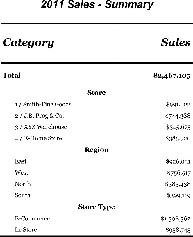
For example, a department store chain’s corporate office may request a Summary report showing store sales by category, along with a corresponding Detail report showing the source of the sales. The Summary report allows the recipient to see the “big picture” of how the corporation is performing. The Detail report allows the reader to better understand the makeup of the summary results and provides the ability to verify that the summary report correctly accounts for the detailed information.

For the purpose of presenting the simpler example first, production of the Detail Report will be presented prior to developing the Summary Report. Figures 1.1 and 1.2 show sample Detail and Summary reports, respectively.

Figure 1.1 Detail

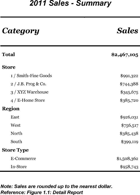
Figure 1.2 Summary

Goals for Creating Complementary Reports

Before getting into the actual implementation of creating complementary reports, it is useful to think about the overall goals and steps needed for achieving these goals.

There are several steps we can implement that will allow for accuracy and ease of use to the reader when analyzing multiple reports. These include:

• A consistent report template

• Consistency of data definitions across reports

• Consistent labels so the end user can easily match items across the reports

• Footnote references clarifying which reports correspond to each other

• Quality checks to ensure that numbers/statistics correspond across reports

Key Steps

For both the Detail and Summary report, three main steps are addressed in the programming: 1) pre-processing the data prior to PROC REPORT, 2) preparing the titles, footnotes, and ODS destination to be used, and 3) using PROC REPORT to create the Detail and Summary reports.

1. Pre-processing (prior to PROC REPORT)

∘ Determine the aspects that are common to both Detail and Summary reports

For this example, the incoming data sets STORE and ECOMM (see Tables 1.1 and 1.2) need to be concatenated, as both Detail and Summary reports display both In-Store and E-commerce sales. The Store Type variable, designating In-Store versus E-Commerce Sales needs to be created since it is not a variable in the existing data sets. The Store Name variable needs to display Store Number before Store Name in the format Store Number / Store Name. Both reports share the title “2011 Sales” and the footnote “Note: Sales are rounded up to the nearest dollar.” The Summary and Detail reports should be based on a common style template for a common look. Both reports, while containing different file names, need to be output to the same file path.

∘ Identify the unique pre-processing steps needed for each individual report

In the case of the Detail report, very little additional processing is needed after the common programming steps are implemented. The data will already be in the structure needed for PROC REPORT. Only one more change is needed, and that is to create a numeric region variable for ordering Region rows in the desired report order.

In the case of the Summary report, Figure 1.2 shows the originally separate variables and their corresponding values Store (STORENAM), Region (REG), and Store Type (TYPE) in one column. The programmer can restructure the data set to map the original variables and values to one variable or column. In addition, a Total row is created as the first row of the report. Because a particular order of rows is desired, variables are created for the specific purpose of assigning numeric order to header and actual data rows. These order variables will be specified later in PROC REPORT as variables that should be used to group and order rows.

2. Titles, Footnotes, and ODS RTF Preparation

The title and footnote text common to both Detail and Summary reports will be assigned to macro variables as one of the pre-processing steps. These macro variables will just need to be referenced in the title and footnote section prior to each PROC REPORT section. Additional title and footnote text specific to each report will be added.

You will need to specify the ODS destination before producing the reports. This includes opening the RTF destination and the specific file path and file name to which the report will be created. In addition, the programmer can assign the ODS style (if different than the default template) that should be applied to the reports. A macro variable (named ODSOPT) specifies ODS options such as orientation (Portrait or Landscape), printing, or suppression of SAS SYSTEM information (dates, page numbers) and other options we wish to apply to the reports. This macro variable is later referenced in an OPTIONS statement.

3. Producing the Report with PROC REPORT

Once the data is in an appropriate format and the RTF destination is designated, we are ready to produce the reports. The Detail report makes use of PROC REPORT’s ORDER option to arrange rows and prevent repeating values, and a BREAK statement with a SUMMARIZE option to sum sales per Store-Region. STYLE options that apply uniquely to the Detail report are specified in the PROC REPORT code, rather than in the PROC TEMPLATE program.

The Summary Report takes advantage of PROC REPORT’s GROUP option to consolidate and establish the order of rows, as well as sum the sales per group. The Summary report also makes use of STYLE options specified directly in the PROC REPORT code.

Source Data

There are two source data sets, each having four variables. The data set STORE contains In-Store sales information, and the data set ECOMM contains E-Commerce sales information. The four common variables are:

• STORENUM (Store Number)

• REG (Region responsible for sales)

• STORENAM (Store Name)

• SALES (2011 Sales)

Tables 1.1 and 1.2 display the STORE and ECOMM data, respectively.

Table 1.1 STORE Data

STORENUM	REG	STORENAM	SALES
1	East	Smith-Fine Goods	$200,310
1	West	Smith-Fine Goods	$189,356
2	East	J.B. Prog & Co.	$89,499
2	West	J.B. Prog & Co.	$44,250
1	North	Smith-Fine Goods	$99,346
1	South	Smith-Fine Goods	$107,220
2	North	J.B. Prog & Co.	$100,171
2	South	J.B. Prog & Co.	$79,465
3	East	XYZ Warehouse	$49,126

Table 1.2 ECOMM Data

STORENUM	REG	STORENAM	SALES
1	East	Smith-Fine Goods	$107,024
1	West	Smith-Fine Goods	$90,033
2	East	J.B. Prog & Co.	$120,050
2	West	J.B. Prog & Co.	$110,631
1	North	Smith-Fine Goods	$88,024
1	South	Smith-Fine Goods	$110,009
2	North	J.B. Prog & Co.	$97,897
2	South	J.B. Prog & Co.	$102,425
3	East	XYZ Warehouse	$159,902
3	West	XYZ Warehouse	$136,647
4	East	E-Home Store	$200,120
4	West	E-Home Store	$185,600

ODS Style Template Used

Both reports are produced in the Output Delivery System (ODS) Rich Text Format (RTF) destination starting with the ODS Journal style template, and modifying the template to a new style named JournalR. The ODS style template is specified prior to the PROC REPORT section in the statement

ods rtf style=journalR file=“{PATHFILENAME}.rtf”;

Programs Used

Though this example presents only two small reports, in reality a list of summary reports along with a list of corresponding detail reports may be requested. Therefore, Detail and Summary reports are created in separate SAS programs. In total, three programs are created and used:

• Ch1Setup.SAS

• Ch1Detail.SAS

• Ch1Summary.SAS

Implementation

Create a Setup Program that Contains Common SAS Code

In this step we create a setup program which contains the code to be used in both Detail and Summary reports. The program includes creating a common style template, macro variable assignments, and data manipulation identified as aspects common to both reports.

Specifically, Ch1Setup.SAS will accomplish the following:

• Set up a common ODS Style Template.

• Create Macro Variables to be used in Report Creation.

• Declare the ODS ESCAPE Character.

• Develop a Macro to Modify Incoming Data for Reports.

Ch1Setup.SAS

** Program Name: CH1Setup.SAS;

** Modify Journal Style Template; ➊

proc template;

define style styles.journalR;

parent=styles.journal;

class fonts /

"DocFont" = ("Georgia", 9 pt) /*Apply to data in cells*/

"EmphasisFont" = ("Georgia", 9 pt, Bold) /*Apply to lines/summaries*/

"HeadingFont" = ("Georgia", 16 pt, Bold Italic); /*Apply to headers*/

class table /

rules=none /*Override Journal default header borders*/

borderwidth=2 pt;

class header /

just=left;

class NoteContent /

font=fonts("EmphasisFont");

class systemtitle /

font_size=16 pt

just=center;

class systemfooter /

font_size=10 pt

just=left

textindent=1.4 in;

end;

run;

** Create Macro Variables to be used in Report Creation; ➋

%let title1 = 2011 Sales;

%let rndfoot = Note: Sales are rounded up to the nearest dollar.;

%let dreffoot = Figure 1.2: Summary Report;

%let sreffoot = Figure 1.1: Detail Report;

%let odsopt = nodate nonumber orientation=portrait missing=“ “;

%let outpath = C:UsersUserMy DocumentsSASBOOKPrograms;

%let template = JOURNALR;

** Set ODS Escape Character; ➌

ods escapechar=“^”;

** Develop Macro to Modify Incoming Data for Reports;

%macro preproc;

/** Concatenate data sets and variables **/

data sales(drop=storenam);

length type $20 storenm $40;

set store(in=instore) ➍

ecomm(in=inecomm);

/** Create Store Type Flags **/

if inecomm then TYPE = “E-Commerce”; ➎

else if instore then TYPE = “In-Store”;

/** Concatenate Store Number with Store Name **/

storenm = catx(" / ",put(storenum,3.),storenam); ➏

run;

%mend preproc;

Ch1Setup.SAS creates a common ODS Style Template

➊ The Detail and Summary reports use a common style template. As a start, the SAS-supplied ODS style template “Journal” is used as the parent style. We name the modified template “JournalR” for this example.

Next, selected style attributes for the style elements Fonts, Table, Header, NoteContent, Systemtitle and Systemfooter are changed via CLASS statements.

• We assign desired font characteristics such as font face, font size, and font weight to various font names (“DocFont”, “EmphasisFont”, and “HeadingFont”) in the CLASS FONTS statement. For example, we change the default Journal Style “HeadingFont”, which applies to the column headers, to ”Georgia", 16 pt., Bold Italic. We change “DocFont”, which applies to data in table cells, to "Georgia", 9 pt.

∘ Note, there is no comma between the font style of “Italic” and the font weight of “Bold,” as in the HeadingFont specification.

∘ We can later reference one of these sets of font characteristics by their corresponding font name when we want these attributes applied to a specific part of the output. For example, "EmphasisFont" is later applied in the CLASS NoteContent statement, informing SAS that this list of font characteristics should be applied to the NoteContent portion of the output (explained further below).

• The CLASS TABLE statement is used to modify the borders of the PROC REPORT table cells. For example, the “rules=none” specification in the Table section removes Journal’s default header borders so that we may apply customized borders in the PROC REPORT code. We thicken the borders to be applied to a 2 pt. width.

• In the CLASS HEADER statement, we left justify the headers.

• The “NoteContent” modifications allow us to obtain the desired font for the COMPUTE block lines and summary rows. We change the NoteContent font from the default to our “Emphasis Font” so the row headers (e.g., “Store” and “Region”) will stand out more in the report.

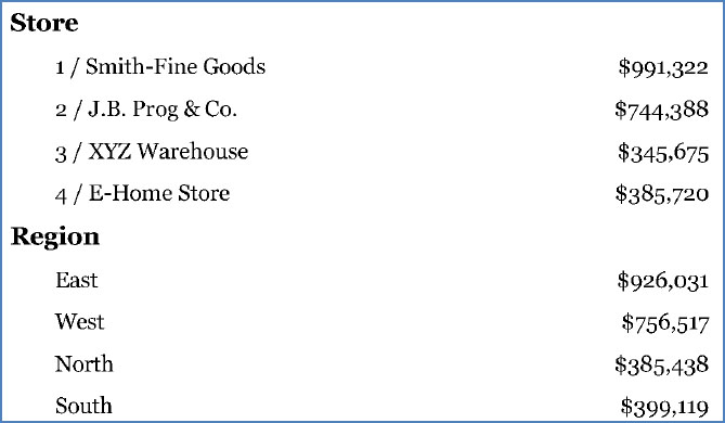
Figure 1.3 displays the default Journal Style NoteContent font (See “Store” and “Region” lines), which is Courier 10 pt. In contrast, Figure 1.4 shows the report with our user-specified “EmphasisFont”, which we chose as (“Georgia”, 9 pt., Bold).

Figure 1.3 Default NoteContent (“Store” and “Region” text)

Description: Figure 1.3 Default NoteContent (“Store” and “Region” text)

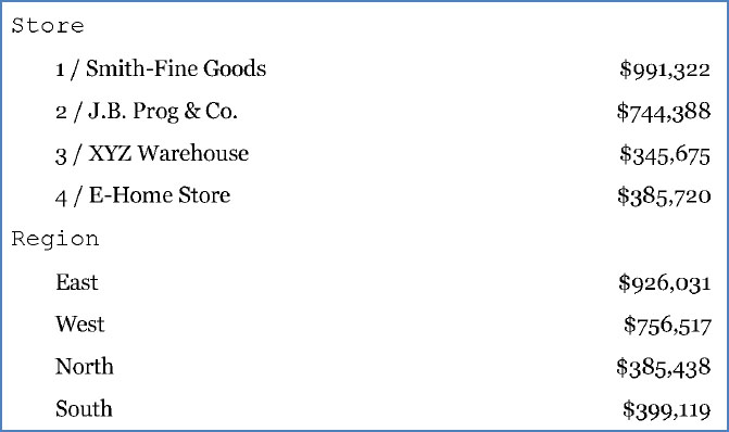
Figure 1.4 NoteContent (“Store” and “Region” text) after our specified EmphasisFont is applied

Description: Figure 1.4 NoteContent (“Store” and “Region” text) after our specified EmphasisFont is applied

The CLASS SYSTEMTITLE and CLASS SYSTEMFOOTER statements are also used to provide template specifications that apply to the Detail and Summary reports. For example, the same Title and Footnote font size and horizontal justification applies to both reports. We provide the instructions for these title and footnote attributes in PROC TEMPLATE so we do not need to specify these in each later title and footnote statement.

For example, The PROC TEMPLATE code

class systemtitle /

font_size=16 pt

just=center;

achieves the same result as

title1 h=16pt j=center "Title goes here";

Likewise, the PROC TEMPLATE code

class systemfooter /

font_size=10 pt

just=left

textindent=1.4 in;

achieves the same result as

footnote1 h=10pt j=left "^S={indent=1.4 in}Footnote goes here";

Recommended books for more information on PROC TEMPLATE and ODS Style Templates can be found in the references section of this book, including (Haworth, Zender, and Burlew (2009) and Smith (2013).

In addition to modifying the ODS Style Template, Ch1Setup.SAS creates macro variables, declares the ODS Escape Character, and prepares the input data set for the Detail and Summary reports.

➋ Ch1Setup.SAS creates macro variables for:

• Common titles – There is one common title, “2011 Sales”, which has been assigned to &TITLE1.

• Common footnotes – There is one common footnote, “Sales are rounded up to the nearest dollar.”, which has been assigned to &RNDFOOT.

• Additional footnotes – The Detail report will reference &DREFFOOT and the Summary Report will reference &SREFFOOT, which contain Figure numbers. These references are placed in the Setup program so any later changes to Figure numbers can be made globally from one location.

• Common options – The SAS system options we want applied to both ODS RTF reports are stored in &ODSOPT.

• Common output path – We want both reports to be stored in “C:UsersUserMy DocumentsSASBOOKPrograms”, which has been assigned to &OUTPATH.

• Common template – Both reports will use the style template, JOURNALR, which has been assigned to &TEMPLATE.

➌ We tell ODS to use the caret character (“^”) as the ODS ESCAPECHAR character value for in-line formatting.

Ch1Setup.SAS also creates the macro PREPROC to handle common data processing:

➍ Concatenate the source data sets STORE and ECOMM

➎ Assign store type variable (based on each source data set – ECOMM or STORE)

➏ Concatenate store names to store numbers

Table 1.3 displays a PROC PRINT of the new data set after calling the PREPROC macro. Note that the data set now contains both In-Store and E-Commerce data, designated by the variable TYPE. STORENM contains each store’s number before the store name.

Table 1.3 PROC PRINT of Data SALES – Result of Macro PREPROC

Type	storenm	STORENUM	REG	SALES
In-Store	1 / Smith-Fine Goods	1	East	$200,310
In-Store	1 / Smith-Fine Goods	1	West	$189,356
In-Store	2 / J.B. Prog & Co.	2	East	$89,499
In-Store	2 / J.B. Prog & Co.	2	West	$44,250
In-Store	1 / Smith-Fine Goods	1	North	$99,346
In-Store	1 / Smith-Fine Goods	1	South	$107,220
In-Store	2 / J.B. Prog & Co.	2	North	$100,171
In-Store	2 / J.B. Prog & Co.	2	South	$79,465
In-Store	3 / XYZ Warehouse	3	East	$49,126
E-Commerce	1 / Smith-Fine Goods	1	East	$107,024
E-Commerce	1 / Smith-Fine Goods	1	West	$90,033
E-Commerce	2 / J.B. Prog & Co.	2	East	$120,050
E-Commerce	2 / J.B. Prog & Co.	2	West	$110,631
E-Commerce	1 / Smith-Fine Goods	1	North	$88,024
E-Commerce	1 / Smith-Fine Goods	1	South	$110,009
E-Commerce	2 / J.B. Prog & Co.	2	North	$97,897
E-Commerce	2 / J.B. Prog & Co.	2	South	$102,425
E-Commerce	3 / XYZ Warehouse	3	East	$159,902
E-Commerce	3 / XYZ Warehouse	3	West	$136,647
E-Commerce	4 / E-Home Store	4	East	$200,120
E-Commerce	4 / E-Home Store	4	West	$185,600

Writing the Detail Report Program

After running the Ch1Setup.SAS program and PREPROC macro for common report features, the only additional preparation needed prior to running PROC REPORT is to create a numeric version of the Region variable to be used in PROC REPORT for ordering rows. The numeric variable will be used in PROC REPORT for arranging the region rows in the order of “East,” “West,” “North,” and “South.”

Detail Report Pre-Processing Code

** %Include Ch1Setup.SAS and Run Pre-processing Macro to Create SALES Data;

** Create Template and macro variables;

%include"C:UsersUserDesktopAPR FINAL CH1_5ProgramsCh1Setup.sas";

** Concatenate and create new data;

%preproc;

** Create Region Informat;

proc format;

invalue region

"East" = 1

"West" = 2

"North" = 3

"South" = 4;

run;

** Create Region Order Variable;

data saledetr;

set sales;

regn=input(reg,region.);

run;

Detail Report: Titles, Footnotes, and ODS RTF Preparation

The Detail report data is now in the desired format for PROC REPORT. The next step is to add the desired titles and footnotes and prepare the ODS RTF destination.

Code for Titles, Footnotes, and ODS RTF Preparation

** Set Page Titles and Footnotes; ➊

title1 "&title1 - Detail";

footnote1 "&rndfoot";

footnote2 "Reference: &dreffoot";

** ODS RTF Preparation;

ods _all_ close ; ➋

options &odsopt; ➌

ods rtf style=&template file="&outpath.detail.rtf" bodytitle; ➍

** {PROC REPORT CODE GOES HERE…};

ods rtf close; ➎

ods html; ➏

title; ➐

footnote; ➑

➊ title1, footnote1, and footnote2 reference previously created macro variables (&TITLE1,

&RNDFOOT, and &DREFFOOT) to apply title and footnote text. The macro variables need to be placed within double quotes so they can be resolved.

The title appears in the RTF output as “2011 Sales – Detail.” The footnotes are printed as “Note: Sales are rounded up to the nearest dollar.” and “Reference: Figure 1.2: Summary Report.”

➋ While closing other destinations is not necessary, the PROC REPORT output is needed only in the RTF destination; therefore the other destinations are closed. If a destination is closed, it is important to remember to reopen any desired destinations once you are ready to print to that destination again, otherwise, you may be wondering why your output is not created.

➌ Reference the ODS options specified in the Ch1Setup.SAS program.

➍ Open the RTF destination.

• Reference the style template specified in the Ch1Setup.sas program (&TEMPLATE)

• Reference the path specified in the Ch1Setup.sas program (&OUTPATH)

• Assign the specific file name for the detail report (“detail”)

• These examples use the BODYTITLE option to place titles and footnotes directly above and below the table rather than in the MS Word headers and footers. With the BODYTITLE option, a title appears once before the top of the table and footnotes appear once after the end of the table. This works for these tables because an entire table fits on one page.

∘ There are methods to place titles and footers directly above and below the table on every page. One method that uses BODYTITLE is shown at: http://support.sas.com/kb/36/288.html (“Sample 36288: Repeating text on an RTF page when the BODYTITLE option is in effect”)

∘ Another method which does not employ BODYTITLE increases the page header margins (with the HEADERY option) and footer margins (with the FOOTERY option) so that the titles and footnotes surround the table.

➎ Close the RTF destination

➏ Re-open any desired printing destinations, in this example HTML

➐, ➑ Reset the titles and footnotes if you don’t want the most recent titles and footnotes carried through to later output

Producing the Report with PROC REPORT

Now that the ODS RTF destination has been opened, we are ready to produce the report. The PROC REPORT code below translates our SALEDETR data (see Table 1.4) into our PROC REPORT output (see Figure 1.5). Note that the data set SALEDETR does not need to be sorted prior to loading it into PROC REPORT. PROC REPORT options will be used to order rows.

Table 1.4 Partial PROC PRINT of SALEDETR Data

type	storenm	STORENUM	REG	SALES	regn
In-Store	1 / Smith-Fine Goods	1	East	$200,310	1
In-Store	1 / Smith-Fine Goods	1	West	$189,356	2
In-Store	2 / J.B. Prog & Co.	2	East	$89,499	1
In-Store	2 / J.B. Prog & Co.	2	West	$44,250	2
In-Store	1 / Smith-Fine Goods	1	North	$99,346	3
In-Store	1 / Smith-Fine Goods	1	South	$107,220	4
In-Store	2 / J.B. Prog & Co.	2	North	$100,171	3
In-Store	2 / J.B. Prog & Co.	2	South	$79,465	4
In-Store	3 / XYZ Warehouse	3	East	$49,126	1
E-Commerce	1 / Smith-Fine Goods	1	East	$107,024	1
E-Commerce	1 / Smith-Fine Goods	1	West	$90,033	2
E-Commerce	2 / J.B. Prog & Co.	2	East	$120,050	1
E-Commerce	2 / J.B. Prog & Co.	2	West	$110,631	2
E-Commerce	1 / Smith-Fine Goods	1	North	$88,024	3
E-Commerce	1 / Smith-Fine Goods	1	South	$110,009	4

Figure 1.5 Partial PROC REPORT Output

Description: Figure 1.5 Partial PROC REPORT Output

The following items are accomplished within the REPORT procedure:

• Specify Variables to be Reported, Left to Right in Desired Order with COLUMN Statement.

• Define Variable Usage, Labels, and Style Elements with DEFINE Statements.

• Summarize Sales after each Region.

• Insert a Blank Line after Each Region.

Detail Report - PROC REPORT Code

** Detail Report;

** Style Report, Column Data and Headers, and Lines; ➊

proc report data = saledetr nowd center split=“|”

style(report)=[cellpadding=0 pt]

style(header)=[vjust=middle borderbottomwidth=2 pt cellheight=.8 in];

** Specify Variables to be Reported, in Desired Order; ➋

column STORENM REGN REG TYPE SALES;

** Define Variable Usage, Labels, and Style Elements; ➌

define STORENM / order "Store" style(column)=[cellwidth=1.4 in

font_weight=bold];

define REGN / noprint order order=internal;

define REG / order "Region" style(column)=[cellwidth=1.4 in

indent=.55 in]

style(header)=[indent=.25 in];

define TYPE / order "Store Type" style(column)=[cellwidth=1.4 in

indent=.3 in]

style(header)=[indent=.1 in];

define SALES / "Sales" style(column)=[cellwidth=1 in just=dec]

style(header)=[just=r];

** Summarize Sales after each Region; ➍

break after REG / summarize suppress

style(summary)=[font_weight=bold

foreground=darkblue];

** Insert a Blank Line Before each Region; ➎

compute before REG;

line “ “;

endcomp;

run;

Key PROC REPORT statements and options used in this example:

➊ Overrides to the STYLE template are applied in the PROC REPORT statement for style elements specific to the Detail report. The overrides are optional and presented primarily for the purpose of demonstrating style overrides to the reader, since they are used throughout the book.

• Cellpadding, the amount of space between the table cell border and its content is set to 0 pt with the STYLE(REPORT)= option. This helps to prevent wrapping, and to decrease the amount of white space within the report so that the full Detail report can fit on one page.

• The header elements and attributes are also modified with the STYLE(HEADER)= option in order to make the report more legible. The headers are centered vertically with the specification VJUST=MIDDLE. A bottom border is created for the headers and is set to a width of 2 pt. The header cell height is increased to .8 inches.

Without the overrides specified in the PROC REPORT statement the Detail report would display as shown in Figure 1.6. In contrast, Figure 1.7 shows the Detail report with the REPORT and HEADER style overrides.

Figure 1.6: Detail Report WITHOUT the STYLE(REPORT)= and STYLE(HEADER)= Overrides

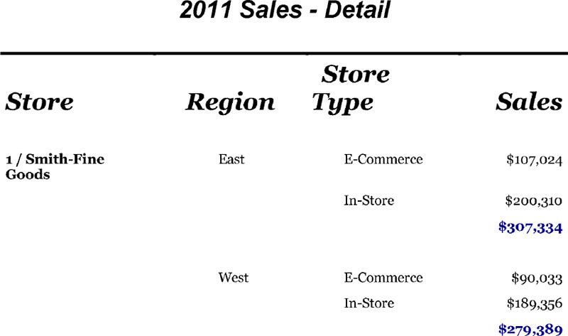
Description: Figure 1.6: Detail Report WITHOUT the STYLE(REPORT)= and STYLE(HEADER)= Overrides

Figure 1.7: Detail Report WITH the STYLE(REPORT)= and STYLE(HEADER)= Overrides

Description: Figure 1.7: Detail Report WITH the STYLE(REPORT)= and STYLE(HEADER)= Overrides

➋ The COLUMN statement specifies the columns to be included left to right. The COLUMN statement also determines the column order in the report, therefore columns are listed in the order in which they should be processed and/or appear in the report (STORENM, REGN, REG, TYPE, and then SALES). Without a COLUMN statement specification, the column order would reflect the physical order of the incoming data set.

➌ We specify variable usage, labels, and style elements in the DEFINE statements.

The ORDER options arrange rows in order of these columns’ values respectively (STORENM, REGN, REG, TYPE). Without the COLUMN and ORDER specifications the rows would not be ordered. SAS would assign the character variables their default usage type, which is DISPLAY, and rows would reflect the physical order of the incoming data set.

• The ORDER usage option without the ORDER= option (e.g., see DEFINE statements for STORENM, REG, TYPE) assumes the default ORDER= option, which is FORMATTED at the time of writing this book. ORDER=FORMATTED orders rows in the order of formatted values, in this case alphanumeric order.

• The ORDER usage option with the ORDER=INTERNAL specification (e.g., REGN) orders rows in the order of unformatted values. Note that in the report, regions are ordered by the unformatted value (1=East, 2= West, 3=North, 4=South) versus alphabetical order. REGN is used for the sole purpose of ordering rows. We suppress the printing of this column with the NOPRINT option.

The ORDER option also:

• Prevents repetition of values over multiple rows (e.g. we want the text “1 / Smith-Fine Goods” to appear only on the first occurrence of this value).

• Allows for use of the BREAK AFTER VARNAME and COMPUTE BEFORE VARNAME before/after each new REG value. (BREAK and COMPUTE based on a BEFORE/AFTER location require GROUP or ORDER usage for that variable).

We apply style overrides in some of the DEFINE statements to override the style template’s attributes for specific columns and headers. This is done with the STYLE(COLUMN)= and STYLE(HEADER)= options.

• For example, for the variable STORENM, we set the column cell width to 1.4 inches. In addition we apply bold font weight to the list of Store Names in the column.

• For the variable REG, we set the column cell width to 1.4 inches, and indent the data in the columns .55 inches. We indent the column header .25 inches.

➍ The sales totals within each Store-Region (summary lines) are generated by the SUMMARIZE option specified in the BREAK statement. Although the ANALYSIS usage option and the SUM statistic are not explicitly specified in the DEFINE statement for Sales, these are applied because ANALYSIS is the default usage for numeric variables, and the SUM statistic is the default behavior for row summaries.

The style of these totals (other than the default italics) are specified in the PROC REPORT statement with STYLE(SUMMARY)=[font_weight=bold foreground=darkblue]

➎ The COMPUTE block creates a blank row before each new value of region (REG) within each store (STORENM).

Writing the Summary Report Program

The Summary Report requires more pre-processing than did the Detail Report to get the data into the desired format for PROC REPORT.

The key Summary Report pre-processing steps include:

• Map separate variables/values to one column for PROC REPORT (CATNAME for “Category” column)

• Derive numeric variables that will be used to assign report row order

Map Separate Variables/Values to One Column for PROC REPORT

Note that in the PROC REPORT output the originally “separate” variable names, STORENAM (Store), REG (Region), and TYPE (Store Type) and their corresponding values appear in one column, “Category.”

Figure 1.8 Originally Separate Variables are Stacked in Category Column

Description: Figure 1.8 Originally Separate Variables are Stacked in Category Column

There are a number of ways to restructure the data in this format. PROC TRANSPOSE is used in this example to map all of the category names and values to a new variable named CATNAME.

Summary Report - Pre-Processing Code

** %Include Ch1Setup.SAS and Run Pre-processing Macro to Create SALES Data;

/** Create Template and macro variables **/

%include"C:UsersUserDesktopAPR FINAL CH1_5ProgramsCh1Setup.sas";

/** Concatenate and create new data **/

%preproc;

** Create TOTAL variable for Total Row in PROC REPORT;

** All records are set to same value (“Total”) for later sum;

data salesumr;

set sales;

total = “Total”;

run ;

** Transpose data to get needed items mapped to Category (CATNAME);

proc sort data=salesumr;

by sales storenum;

run;

proc transpose data=salesumr out=salesum2(rename=(col1=catname));

by sales storenum;

var total storenm reg type;

run;

Figure 1.9 displays a partial PROC PRINT of the transposed data, sorted by _NAME_ and STORENUM. A sort is not needed but is performed so you can better see how the sales data will eventually translate into sums. The variables that you want to end up in one column (COL1, renamed to CATNAME) are specified in the PROC TRANSPOSE VAR statement. In the partial PROC PRINT (Figure 1.9) you can see that _NAME_ contains our original variable names, for example STORENM. CATNAME contains the values for these items.

Figure 1.9 Partial PROC PRINT of Transposed Data

Description: Figure 1.9 Partial PROC PRINT of Transposed Data

The transposed data rows above are not yet in the desired order for our Summary Report, but you can get the idea that the data is now structured so the observations within groups can be summed, as in Figure 1.10.

Figure 1.10 Sale Summed in Summary Report

Description: Figure 1.10 Sale Summed in Summary Report

Assign Report Order to Variables

Two numeric variables, CATORD and SUBCTORD, are created specifically for ordering data later on in the REPORT procedure.

CATORD will be used to order categories and to insert blank rows after each group. Total is the first category (given a value of 0). Store and its associated values (1 / Smith-Fine Goods, 2 / J.B. Prog, etc.) are the second category (given a value of 1). Region and its associated values are the third category (given a value of 2), and so on.

SUBCTORD will be used to order rows within each category. Within Store, stores will be sorted by Store Number (1, 2, 3, and 4). Within Region, East will be shown first, then West, etc.

Table 1.5 shows the mapping of rows to CATORD and SUBCTORD which will translate into row order in the Summary Report.

Table 1.5 Derive CATORD and SUBCTORD for Ordering Rows

catname	catord	subctord
Total	0	0
1 / Smith-Fine Goods	1	1
2 / J.B. Prog & Co.	1	2
3 / XYZ Warehouse	1	3
4 / E-Home Store	1	4
East	2	1002
West	2	1003
North	2	1004
South	2	1005
E-Commerce	3	1007
In-Store	3	1008

Code for Creating Ordered Variables

** Informats for Summary Report; ➊

proc format;

invalue catord

“TOTAL” = 0

“STORENM” = 1

“REG” = 2

“TYPE” = 3;

invalue rowlabl

"Total" = 0

"Region" = 1

"East" = 2

"West" = 3

"North" = 4

"South" = 5

"Store Type" = 6

"E-Commerce"= 7

"In-Store" = 8;

run;

data salesum2;

set salesum2;

** Create CATORD for ordering groups of rows in PROC REPORT; ➋

catord = input(upcase(_name_),catord.);

** Create SUBCTORD to order sub-category rows in PROC REPORT;

if catord = 0 then subctord = 0; ➌

else if catord = 1 then subctord = storenum; ➍

else subctord = input(catname,rowlabl.) + 1000; ➎

run;

➊ Informats are created to reflect the desired row reporting order of categories and subcategories.

➋ A CATORD value is assigned for every row.

➌ Note that the “Total” rows (where CATORD=0) are assigned a SUBCTORD value of 0 to ensure “Total” is reported before the first Store Number (1).

➍ For Store (names) the assumption is that the list of stores will grow, and in future runs of our program we don’t want to have to add new formats to our list each time new stores are added or a store number changes. Therefore, rather than using informats to assign stores a number, an assignment statement that captures store number is used.

➎ For the shorter and/or finite lists for Region and Store Type, an informat is used to assign SUBCTORD. Note the “+ 1000” added to the Region and Store Type values (because these variables occur after STORE) to ensure these rows are ordered after the last store number, which we expect to increase over time.

Summary Report: Titles, Footnotes, and ODS RTF Preparation

The data set is now in the needed structure for PROC REPORT. The next step is to prepare titles, footnotes, and ODS RTF setup.

Code for Titles, Footnotes, and ODS RTF Preparation

** Titles and Footnotes;

title1 "&title1 - Summary";

footnote1 "^S={indent=2 in}&rndfoot";

footnote2 "^S={indent=2 in}Reference: &sreffoot";

** ODS RTF Setup;

ods _all_ close ;

options &odsopt;

ods rtf style=&template file="&outpath.salessum.rtf" bodytitle;

** {PROC REPORT CODE GOES HERE…};

ods rtf close;

ods html;

title;

footnote;

The process for applying titles and footnotes is the same as that for the Detail Report section. We’re simply changing some of the titles and footnotes that apply to the Summary report. Beside the verbiage, we change the indentation of the Summary report footnote (from 1.4 inches to 2 inches) to align with this smaller table. The style override is applied by inserting the inline formatting function, ^S={indent=2 in} within the quotation marks around each footnote. The title appears in the RTF output as “2011 Sales – Summary”. The footnotes appear as “Note: Sales are rounded up to the nearest dollar.” and “Reference: Figure 1.1: Detail Report”.

The ODS RTF statements are the same as for the Detail report section with the exception of the file name (salessum) specification.

Producing the Report with PROC REPORT

Now that our data is in the desired structure, a small amount of PROC REPORT code will translate our SALESUM2 data (Table 1.6) into our Summary Report (Figure 1.11).

Table 1.6 Partial PROC PRINT of Final Sales Summary Data

catname	catord	subctord	SALES
Total	0	0	$44,250
Total	0	0	$49,126
Total	0	0	$79,465
Total	0	0	$88,024
Total	0	0	$89,499
Total	0	0	$90,033
Total	0	0	$97,897
Total	0	0	$99,346
Total	0	0	$100,171
Total	0	0	$102,425
Total	0	0	$107,024
Total	0	0	$107,220
Total	0	0	$110,009
Total	0	0	$110,631
Total	0	0	$120,050
Total	0	0	$136,647
Total	0	0	$159,902
Total	0	0	$185,600
Total	0	0	$189,356
Total	0	0	$200,120
Total	0	0	$200,310
1 / Smith-Fine Goods	1	1	$88,024
1 / Smith-Fine Goods	1	1	$90,033
1 / Smith-Fine Goods	1	1	$99,346
1 / Smith-Fine Goods	1	1	$107,024
1 / Smith-Fine Goods	1	1	$107,220
1 / Smith-Fine Goods	1	1	$110,009
1 / Smith-Fine Goods	1	1	$189,356
1 / Smith-Fine Goods	1	1	$200,310
2 / J.B. Prog & Co.	1	2	$44,250
2 / J.B. Prog & Co.	1	2	$79,465
2 / J.B. Prog & Co.	1	2	$89,499
2 / J.B. Prog & Co.	1	2	$97,897
2 / J.B. Prog & Co.	1	2	$100,171
2 / J.B. Prog & Co.	1	2	$102,425
2 / J.B. Prog & Co.	1	2	$110,631
2 / J.B. Prog & Co.	1	2	$120,050
3 / XYZ Warehouse	1	3	$49,126
3 / XYZ Warehouse	1	3	$136,647
3 / XYZ Warehouse	1	3	$159,902

Figure 1.11 Transformation of PROC PRINT to PROC REPORT Output

Description: Figure 1.11 Transformation of PROC PRINT to PROC REPORT Output

Summary Report - PROC REPORT Code

{Add to the PROC FORMAT section…} ➊

value rowheadr

0 = " "

1 = "Store"

2 = "Region"

3 = "Store Type";

** Summary Report;

proc report data = salesum2 nowd missing center split=“|”

style(header)=[vjust=bottom cellheight=.55 in]

style(lines) =[vjust=top just=l font_size=10 pt]

OUT=PRSSUM; ➋

column catord subctord catname sales;

define catord / group order=internal noprint; ➌

define subctord / group order=internal noprint; ➌

define catname / group order=internal "Category" ➌

style(column)=[cellwidth=2.4 in];

define sales / "Sales" style(column)=[cellwidth=1.6 in just=r]

style(header)=[just=r];

** Change Total Row Style Attributes and Indent Subcategory Row Headers; ➍

compute catname /char length=30;

if catname ne “Total” then

call define(“catname”,”style”,”style={indent=.25 in}”);

else

do;

call define(_row_,”style”,”style={bordertopwidth=2 pt

cellheight=.5 in vjust=middle

font_size=10 pt

font_weight=bold}”);

end;

endcomp;

** Print Category Row Headers; ➎

compute before catord;

line catord rowheadr.;

endcomp;

run;

PROC REPORT will be able to translate our Table 1.6 data structure into Figure 1.11 by…

➊ Adding a format to assign the values we would like to see in the report for the main row headers “Store“,“Region“,“Store Type“). The “Total” row does not get a row header.

➋ Applying style attributes to the column headers and COMPUTE block lines.

• The column header style override (accomplished with STYLE(HEADER=) option) adjusts the vertical justification, placing the header text at the bottom of the cell. The cell height is reset to .55 inches.

• The COMPUTE block line statement style override (accomplished with STYLE(LINES=) option) resets the vertical justification of the Row headers to be at the top of the cell, and horizontal justification to be left. The font size is set to 10 pt. Note that without the JUST=L style override for LINES, the row headers would be centered as shown in Figure 1.12.

Figure 1.12 - Summary Report Without JUST = L Style Override for LINES

Description: Figure 1.12 - Summary Report Without JUST = L Style Override for LINES

➌ We consolidate rows and sum the ANALYSIS variable SALES by applying the GROUP option to CATORD, SUBCTORD, and CATNAME. In this context, “Consolidate” means to collapse a group of rows into a summary row. For example, the store “1 / Smith-Fine Goods” gets one row showing its summed sales. The store “2 / J.B. Prog & Co.” gets one row showing its summed sales, and so on.

While the primary reason for using the GROUP option here is to consolidate rows, the option also orders the rows for us. The COLUMN statement’s specified order of columns (CATORD SUBCTORD CATNAME) along with the GROUP option specified in the DEFINE statements arrange rows in order of these variables’ values respectively. The GROUP option also allows for use of the COMPUTE before each new CATORD value.

➍ We use a COMPUTE block to indent the rows showing levels of variables, and leave the variable names (shown as row headers) un-indented.

CALL DEFINE statements are used to conditionally apply style attributes to the “Total” row versus the row headers. Note that CALL DEFINE can be used only in a COMPUTE block that is attached to a report item. In this case, our report item CATNAME is already part of the input data set. We COMPUTE the variable CATNAME so we can apply the CALL DEFINEs, but we still define CATNAME’s usage as GROUP so we can consolidate rows.

• In order to make the Total sales row stand out, we increase the font size, font weight (bold), and cell height where CATNAME equals “Total”. A top border is added and the cell text is centered vertically (“VJUST=MIDDLE”). Because we want these style attributes applied to the entire “Total” row, we identify _ROW_ (without quotation marks) as the item to which the CALL DEFINE attributes should be applied, as in “call define(_row_,……..)”.

• The subcategory row headers (e.g., “East,” "West,” “North,” and “South”) are indented .25 inches. (The subcategories occur where CATNAME does not equal “Total”.) In the case of the subcategory rows we only apply the indentation to the CATNAME column. Therefore the CALL DEFINE is applied only to the column “CATNAME”. The column must be enclosed in quotation marks, as in call define(“catname”, ……..)”.

➎ A COMPUTE block LINE statement is used to print the appropriate row header text (“Store”, “Region”, and “Store Type”) before each new value of CATORD.

For the reader’s reference, the output data set created by the PROC REPORT code is shown in Table 1.7. The optional output dataset, named PRSSUM here, is created with the OUT= option in the PROC REPORT statement.

It is worth noting that the COMPUTE BEFORE results are represented differently in the output data set (Table 1.8) than in the printed report (Figure 1.13). Table 1.7 notes some of these differences.

Table 1.7 COMPUTE BEFORE Representation in Output Data Set Versus Printed Report

Output Data Set PRSSUM (Table 1.8)	Printed Report (Figure 1.13)
The COMPUTE block LINE statement results do not appear in the output data set.	The COMPUTE block LINE statements display as row headers, “Store,” “Region,” and “Store Type” corresponding to the CATORD values 1 through 3 respectively.
COMPUTE BEFORE CATORD generates a summary line BEFORE each distinct value of catord, in which the analysis variable SALES is summarized for each catord group in the data set.	If we want these summary sales rows to print in the printed report, we need a BREAK statement with a / SUMMARIZE option. Since this is not desired for the printed report, a customized summary line is created with a LINE statement.
The output data set contains an automatic internal variable named “_BREAK_.” In this case, _BREAK_ is populated with the value “catord” due to the COMPUTE BEFORE CATORD statement.	This variable is not a report item and is not printed.
CATORD and SUBCTORD are still part of PROC REPORT’s data set in spite of the NOPRINT option.	CATORD and SUBCTORD variables do not display in the printed report due to the NOPRINT option.

Table 1.8 PROC PRINT OF PRSSUM Data Set

catord	subctord	catname	SALES	_BREAK_
0			$2,467,105	catord
0	0	Total	$2,467,105
1			$2,467,105	catord
1	1	1 / Smith-Fine Goods	$991,322
1	2	2 / J.B. Prog & Co.	$744,388
1	3	3 / XYZ Warehouse	$345,675
1	4	4 / E-Home Store	$385,720
2			$2,467,105	catord
2	1002	East	$926,031
2	1003	West	$756,517
2	1004	North	$385,438
2	1005	South	$399,119
3			$2,467,105	catord
3	1007	E-Commerce	$1,508,362
3	1008	In-Store	$958,743

Figure 1.13 PROC REPORT Output

Description: Figure 1.13 PROC REPORT Output

Chapter 1 Summary

This chapter showed steps the programmer can implement that will allow for accuracy and ease of use to the reader when analyzing multiple reports. These include:

• A consistent report template

∘ Example: Use of the same ODS Style template, with like style elements and attributes across reports

• Consistency of data definitions across reports

∘ Example: Macro variables and macro used to merge E-Commerce and In-Store data, creation of the TYPE variable to designate these items, and concatenation of Store Name with Store Number

• Consistent labels across the reports

∘ Example: titles, footnotes, headers, value labels (Store Names, the Regions, Store Type values)

• Footnote references clarifying which reports correspond to each other

∘ Example: The Detail report’s footnote “Reference: Figure 1.2: Summary Report” indicates that these two reports should be used in conjunction with one another. Likewise, the Summary report footnote references Figure 1.1: Detail Report.

• Check that numbers/statistics correspond across reports

∘ Example: All of the “1 / Smith-Fine Goods” sales in the Detail report sum to $991,322, the total “1 / Smith-Fine Goods” sales reported in the Summary report.

..................Content has been hidden....................

You can't read the all page of ebook, please click here login for view all page.

Table of Contents for Chapter 1: Creating Complementary Reports

Create new playlist

Sign In

Sign Up

Chapter 1: Creating Complementary Reports

Introduction

Example: Department Store Summary and Detail Reports

Goals for Creating Complementary Reports

Key Steps

Source Data

ODS Style Template Used

Programs Used

Implementation

Create a Setup Program that Contains Common SAS Code

Ch1Setup.SAS

Writing the Detail Report Program

Detail Report Pre-Processing Code

Detail Report: Titles, Footnotes, and ODS RTF Preparation

Code for Titles, Footnotes, and ODS RTF Preparation

Producing the Report with PROC REPORT

Detail Report - PROC REPORT Code

Writing the Summary Report Program

Map Separate Variables/Values to One Column for PROC REPORT

Summary Report - Pre-Processing Code

Assign Report Order to Variables

Code for Creating Ordered Variables

Summary Report: Titles, Footnotes, and ODS RTF Preparation

Code for Titles, Footnotes, and ODS RTF Preparation

Producing the Report with PROC REPORT

Summary Report - PROC REPORT Code

Chapter 1 Summary

Table of Contents for
Chapter 1: Creating Complementary Reports