
![]()
Introducing Big Data Analytics
By this time you have read 12 chapters on the topic of business analytics and can now appreciate the theories and practices that make up this domain. But the learning never ends, especially in a fast-growing area like this one. By now, you might already be aware that big data is catching up in popularity very quickly. A fast-growing number of organizations, notably online ones with a large amount of visitor traffic, are generating an unprecedented amount of data daily, which is almost impossible to handle with classic techniques.
We discussed this a bit in Chapter 1, and in this last chapter of the book, we expand your understanding so that you get a feel of the big data domain and understand what tools and techniques are used by the experts working in this field.
Traditional Data-Handling Tools
In your day-to-day work, you might use one or more of the following tools:
- Text editor/Notepad: For modifying small amounts of data
- Microsoft Excel: For simple and medium calculations
- Microsoft Access/SQL: For storing and querying relational data
- SAS/R: For advanced analytics
- Tableau/QlikView: For data visualization and reporting
Have you ever tried to open a 2GB file using Notepad? Have you ever worked with an Excel file of 4GB? Is it possible to create a 4GB Excel file in the first place? How much time does it take to query a 10GB database? Have you ever performed any analytics operation like regression on a 20GB data set? Can SAS or R handle 20GB data with equal efficiency as relatively smaller data sets? We’ll present some examples to give you a feel of where we are coming from.
About 245 million active customers and members visit Walmart in 11,000 stores under 71 banners in 27 countries, which includes its e-commerce web sites (http://corporate.walmart.com/our-story/). Imagine that Walmart wants to know its customers’ buying patterns for the last month. Let’s try to get a rough estimate of how much data is generated by Walmart in a month. The following calculations may give a conservative estimate:
(245,000,000 customers) × (2 visits per month) × (20 items bought per visit) = 9,800,000,000 rows
There might be as many as 9.8 billion rows in one month. For each row, Walmart must be tracking details such as the date stamp, item ID, number of items, item price, net price, and so on. Again, using a conservative approach, let’s imagine that there are a minimum of six columns in each such row. What will the size of the file be with 9.8 billion rows and 6 columns? Generally speaking, for a CSV or TXT file with 10,000 rows and 6 columns per row, the approximate file size may be around 210KB. Based on this, the size of a similar file with 9.8 billion rows will be approximately 196GB. And this is just one month’s conservative estimate for only the billing transactions. Envisage the data for customers’ previous purchases, demographics data, product details, store details, and so on. A basic file that needs be considered for any customer analytics will be much larger than our estimate of 160GB.
Let’s imagine that Facebook (or a social media network of that size) wants to build an effective online advertisement (ad) engine. Depending upon its user profiles, Facebook wants to display the most relevant ad on each web page. Or it wants to improve the Facebook feeds. Let’s try to estimate the minimum amount of data generated by Facebook in a month.
Facebook has more than 1 billion users. There are 864 million daily active users. Just for the sake of simplicity, let’s treat the user activities such as share, likes, status updates, picture uploads, login and logout, and so on, as one activity. Consider the following conservative calculations:
(864,000,000 customers) × (30 activities per month) = 25,920,000,000 rows
A file with 25.92 billion rows and 6 columns (for example) may be on the order of 510GB. Facebook may need to handle at least this much amount of data if it wants to do any meaningful analytics for its ad engine. And this is just a simulated example to give you a feel of the amount of data involved in the process.
Note that the Walmart and Facebook estimates are conservative as far as the amount of data involved. The actual data size involved might be much bigger. Some real-life business scenarios might require you to handle petabytes of data. What is a petabyte? Refer to Table 13-1.
Table 13-1. Units of Data
|
Unit Measure |
Conversion |
|---|---|
|
1GB Gigabyte |
1024MB |
|
1TB Terabyte |
1024GB |
|
1PB Petabyte |
1024TB = 1024GB × 1024GB = 1,048,576GB |
As an example, consider that a typical DVD stores about 4.7GB of data. To store 1PB of data, you would need 223,101 DVDs.
Examples of the Growing Size of Data
The real-time data produced and analyzed by some enterprises is sometimes even beyond our imagination.
- Walmart has a database with more than 2.5 petabytes of data.
- Facebook handles 300 petabytes of data daily.
- Google handles nearly 200 petabytes of data every day.
- NASA stores and processes around 32 petabytes of climate data and related simulations.
- Large Hadron Collider (LHC) at CERN produced 30TB of data in 2012.
By now, it may be clear that you can’t handle these large volumes of data using traditional tools. Does big data really mean a large data set? What is the definition of big data?
What Is Big Data?
There is no standard definition for big data. The following are a few definitions that are floating around the Internet:
- Any data set that is difficult to handle with conversional or traditional data-processing tools is called big data.
- Data that is difficult to capture, store, process, search, query, transfer, analyze, and visualize is called big data.
- Big data is a complex, varied, rapidly growing, and huge data set that requires new architecture, techniques, and algorithms to analyze it.
- Big data is a data set that can be analyzed and mined for insights, but because of its size, complexity, and growth rate, traditional tools fail to process it.
The following two sections basically revise what we discussed in Chapter 1.
The Three Main Components of Big Data
Big data is not just about the size, though the volume of the data plays a big role in the failure of traditional tools while handling it. There are three main components of big data: volume, verity, and velocity. The traditional methods and tools have their own limitations in processing the data. The following bullets shed some more light on each of these characteristics:
- Volume: The sheer size of the data, in big data analytics, is so large that it becomes almost impossible to process. So far we have mentioned several examples, and to add some more examples, transactional data from credit card companies, call data from a cell phone company, and billing data from a big retailer like Amazon fall under this category. Size is considered the first characteristic of defining big data.
- Variety: The type of data that we are generating these days is limited not just to structured numerical tabular data. Examples are audio files from telecom companies, video files from numerous closed-circuit cameras, and blog data from many web sites. All these are nonconventional types of data. Other data in this category includes text, numerical data, sequences, time series, multidimensional arrays, XML, still images, and social media data. These types of data may come pooled with the conventional data. Preparing this type of data for analysis is obviously not simple.
- Velocity: Data is growing day by day at a rapid pace. In some situations, data keeps growing so fast that we do not have enough time to analyze it. Imagine a Formula One scenario. We invariably have some sensors placed in each super car. The data collected by these sensors is analyzed so as to give some suggestions for improvements for the next round. We can’t take, for example, three months to transform the data, prepare it for analysis, build a model, and finally validate it so that some useful recommendations can be made based on this analysis. All this needs to happen well before the next lap starts. This type of analytics even uses real-time data streaming from car sensors. Table 13-2 compares big data to conventional data. It’s reproduced from Chapter 1 for a ready reference.
Table 13-2. Big Data vs. Conventional Data
|
Big Data |
Normal or Conventional Data |
|---|---|
|
Huge data sets. |
Data set size in control. |
|
Unstructured data such as text, video, and audio. |
Normally structured data such as numbers and categories, but it can take other forms as well. |
|
Hard-to-perform queries and analysis. |
Relatively easy-to-perform queries and analysis. |
|
Needs a new methodology for analysis. |
Data analysis can be achieved by using conventional methods. |
|
Need tools such as Apache’s Hadoop, Hive, HBase, Pig, Sqoop, and so on, to handle big data. |
Tools such as SQL, SAS, R, and Excel alone may be sufficient to handle traditional data. |
|
Raw transactional data. |
The aggregated, sampled, or filtered data. |
|
Used for reporting, basic analysis, and text mining. Advanced analytics is only in a starting stage in big data. |
Used for reporting, advanced analysis, and predictive modeling. |
|
Big data analysis needs both programming skills (such as Java) and analytical skills to perform analysis (as of today). |
Analytical skills are sufficient for conventional data; advanced analysis tools don’t require expert programing skills. |
|
Petabytes/exabytes of data. Millions/billions of accounts. Billions/trillions of transactions. |
Megabytes/gigabytes of data. Thousands/millions of accounts. Millions of transactions. |
|
Generated by big financial institutions, Facebook, Google, Amazon, eBay, Walmart, and so on. |
Mostly generated by small enterprises. |
Now you know that big data is complex, huge, and rapidly growing. Also, it’s almost impossible for the traditional tools to process this kind of data. Why do we really need to analyze big data? Can’t we simply use aggregated data or sample data sets and stick to the traditional techniques and tools? What are the applications of big data analytics in real life? The following section answers all these questions.
Applications of Big Data Analytics
Not long ago, it was not a common practice to send soft copies of data. We used to mail all the data in the form of hard copies, arranged in files and bundles. With the advent of computers, smartphones, and other devices, we are able to store and process huge amounts of data. Now the data is growing in an exponential manner. There are already some smart companies that are using this vast amount of available data to their benefit. Here are some examples:
- E-commerce retailers: Online retailers such as Amazon and eBay need to handle the millions of customers online who are purchasing thousands of products. They analyze petabytes of data every day to recommend the right products, improve searches, and improve service quality. Performing big data analytics reveals so many customer insights such as customer lifetime value, customer loyalty, product popularity, and so on.
- Online entertainment industry: Sites such as Netflix are using big data analytics to understand customer sentiments. They are analyzing big data for movie recommendations and even for ticket pricing based on the demand.
- Automobile industry: Car manufacturers collect data from millions of vehicles worldwide using sensors. Because of the data’s sheer size, its variety, and the pace with which it accumulates, it falls under the big data category. This data is used in understanding the maintenance issues with the models, strong and weak points in a particular model, customer driving habits, causes of accidents, suggestions on quality improvements, and so on.
- Telecom industry: In addition to the billing and complaints data, telecom companies also maintain call detail record data (CDR) and text messages data. These days a smartphone is an integral part of human life. By analyzing CDR data, one can get some vital analytics on people’s habits such as sleeping hours, most active hours, office hours, driving time, and so on. This data can be utilized by the civic authorities in planning and managing cities by setting up the right infrastructure at places. Numerous such uses can be found once the analytics models are in place.
- Online social media industry: One of the most popular users of big data is the social media industry. Social networking sites such as Facebook, Google+, Twitter, and LinkedIn generate petabytes of data every day. They analyze this data for friends’ recommendations, advertisement management, feed management, and so on.
These are just a few examples. In fact, big data analytics is also used in the healthcare industry in drug invention. The industry uses simulated data rather than conventional lab experiments. Another use of big data is video analytics for self-driving cars. In addition, search engines are using big data in indexing, searching, and querying. Big data is used in politics too. Many popular politicians have used big data analytics along with focused e-mail campaigns to get an estimate of their chances of winning. So, as you see, the uses and possibilities are beyond one’s imagination.
Now that you are familiar with the big data introductory concepts, we will discuss some more applications in the form of the following questions, many of which were considered as far-fetched ideas just a few years ago:
- How about getting some real-time recommendations and discounts (maybe on a cell phone) when we drop an item into a cart in a supermarket?
- How about a city with 100 percent self-driven cars?
- Can we wear some glasses and get complete information of the objects that we see through those glasses?
- Can we predict the result and change in the winning probability of a football match as it happens?
- In real time can we control the traffic and better manage it during the peak hours?
- Can we create a robot that can understand the human language and reply in real time?
- Can we have a smartphone that realizes our blood pressure levels? Can we have an app that rings an alarm at the time of a heart attack?
- Can we analyze a call center’s historic voice data and automatically resolve customer queries instead of an agent physically answering a question?
All this looks too advanced to be true. But these are all possibilities with big data. Unfortunately, big data can’t be processed using traditional tools, old techniques, or typical algorithms; we need an alternative solution.
The Solution for Big Data Problems
The reason for the failure of traditional data-processing techniques when analyzing big data is apparent. The conventional tools take the complete data set as one unit. In that way it would be painful to handle the data in the orders of petabytes. Sometimes it’s not even possible to save big data files on one machine. We need gigantic supercomputers with multiple processors to handle big data using one machine. A supercomputer is not a simple machine; it costs millions of dollars. The solution to the big data challenge is to connect multiple computers using computer networks (such as LANs), writing the code in such a way that it is separately understood and executed at each computer and the results are finally assembled as one output. This technique is called distributed computing.
Distributed Computing
Even today, the need of high-computing power is sometimes listed as a major limitation in dealing with big data. Distributed computing appears to work well in these situations. It works on the principle of “divide and rule.” Instead of considering a huge data set as a single unit, you can it cut into pieces or small data chunks. You can then save these relatively smaller pieces of data on an array or network of computing devices. Each computer in this network is called a node. Distributing the data onto a cluster setup is the first part of distributed computing. The second part is to adapt the code for this kind of cluster of computers. The following points summarize the distributed computing approach for dealing with big data:
- Modify the overall problem into smaller tasks and execute smaller tasks on an array of individual computers. That translates to dividing the data into smaller blocks and storing the blocks on individual nodes in the cluster.
- Collate the results from all the individual machines and deliver a consolidated output.
Let’s take the same example of Facebook or a similar networking site. In a day there are billions of activities on this social networking web site. Say you want to get the number of status updates in a day. Imagine that the overall status updates file is 500GB. The following could be the simple SQL code to calculate the total count of status updates:
Select count(*) from feb_status /* feb_status is the status updates data set name */
This code will treat the whole 500GB file as one unit, and it might take an unusually long time. What if you take a network of 20 computers and divide this 500GB file into 10,000 pieces of 50MB each? You can store these 10,000 individual data chunks on 20 computers. By doing so, you are distributing the one big task of computation onto 20 machines. Each computer can locally calculate the number of status updates, and then the count data can be totaled to get the desired consolidated number of status updates. All 20 machines are working in parallel on independent chunks of data. If the overall computing task takes 20 hours using the traditional method and a single machine, it might be natural to expect that with this divide-and-rule policy, it will take only an hour or less to complete. In practice, using distributed computing, it will take much less than an hour to complete the whole task.
A supercomputer also could have done the same task efficiently. But, generally speaking, even medium and small enterprises can afford a cluster of 20 PCs when compared to the prohibitive costs of one large supercomputer. Moreover, 20 PCs can be put to other commercial use when there are no big data files to be analyzed. A supercomputer, on the other hand, will make sense only for high-end tasks, which might not be available all the time.
The programing model wherein you divide a big computing task into smaller tasks and collate the intermediate results to generate the ultimate result is called the MapReduce programming model.
What Is MapReduce?
In distributed computing, the aim is to solve a global problem. You write a program to divide this global task into smaller ones and finally assign the pieces to individual machines forming a cluster. This divide program is called a map function. Once you are done with the local machine tasks, you then write another program to sum up the results from the individual map functions to generate a final consolidated result. This consolidation function is termed a reduce function. We discuss each function in the following sections.
Map Function
The map function is locally executed on all individual chunks of data. The result of a map function comes in the form of a key-value pair. These key-value pairs, from different map functions, carry the intermediate results. Generally any individual map function is similar to the overall task. The only difference is the size, which is considerably smaller for the map function. The outputs of map functions are used as the inputs of the reduce function.
Reduce Function
The reduce function takes the intermediate results from the map functions and creates the final output. The key-value pairs generated by the map functions is sorted and aggregated in the reduce function. The reduce function doesn’t act on the individual pieces of data. In fact, it has no interaction with the original input data, which was fed only to the map functions.
Figure 13-1 shows a reduce diagram that explains the overall MapReduce programming model that is used for handling big data. It’s a cost-effective and efficient model of processing big data.
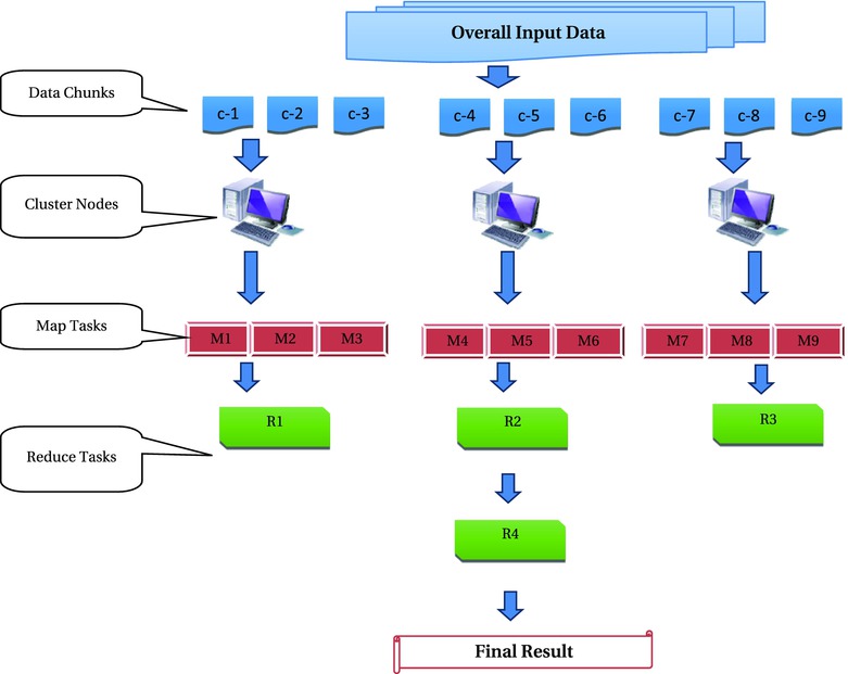
Figure 13-1. How MapReduce handles big data problems
In addition to the MapReduce programming model, the following processes also need your attention:
- Cluster setup: You set up a cluster by creating a network of individual machines. You may need to get the help of a system admin for setting up a cluster.
- Work assignment: Choose some nodes as slaves and assign the map tasks followed by the reduce task. You need to write a separate function to assign the work to individual nodes.
- Task scheduling: Create a master node, which will keep track of all the MapReduce tasks, meaning the scheduling. You can’t start with a reduce task. That doesn’t mean you need to wait until all the map tasks are completed, though. You may need to write some separate code for scheduling the tasks.
- Load balancing: There will be challenges; say one system in the cluster is slow. Some nodes in the cluster may have a good configuration. To achieve the desired efficiency, you need to assign the tasks based on the capacity of nodes. This may require you to write functions for load balancing as well.
- Fault tolerance: What if one of the nodes shuts down suddenly? Is there any way you can retrieve the data in that node? Maybe it is a good idea to replicate that specific load chunk onto a different machine and use it as a backup. So, you may need to take care of replication also while distributing the data.
It appears that MapReduce is a solution to big data problems, but, as you see, there are so many complicated interconnected tasks that make it difficult for an average programmer to try. You need multiple skills to solve a big data problem using the MapReduce programming model. It would be great if you have a readymade framework that takes care of setting up a cluster, adding and deleting nodes, assigning work, scheduling tasks, load balancing, fault tolerance, and so on. Apache Hadoop is the one such popular framework. Hadoop is open source, and it’s a windfall for those who want to focus on MapReduce.
The solution for the challenges of several issues of distributed computing using the MapReduce programing model is the Hadoop framework. The Hadoop framework is an open source tool, built on the Linux operating system.
Hadoop is a framework. It is a simplified platform to write and execute MapReduce and other big data tasks. Hadoop has two major components: the Hadoop distributed file system (HDFS) and MapReduce. We go into the details of these two components in the following sections.
Let’s be clear on a few facts.
- Hadoop is not a database.
- Hadoop is not a synonym of big data.
- Hadoop is not a programing language.
Hadoop Distributed File System
In the world of distributed computing and MapReduce, there should not be any abnormally big files. All big files will be cut into pieces. The file system in Hadoop is called the Hadoop distributed file system. Every file in that system will be 64MB or less. If you transfer any file from outside to HDFS, it will be broken into pieces of 64MB. In the case of a cluster, HDFS will cut the files into pieces and distribute them to the different nodes within the cluster. You can imagine HDFS as a chopper that cuts the data into small chunks. With it, developers do not need to worry about the division and distribution of data. All that you need to do is copy the file from the local file system to HDFS. In fact, HDFS will even take care of details such as the data block locations. There will be replication of data blocks; if one system goes down, then replicated data blocks will be used. Figure 13-2 shows how HDFS distributes the data.
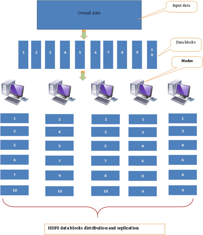
Figure 13-2. How HDFS distributes data
In Figure 13-2, each block has been replicated three times. By default each block size will be 64MB, and it will be replicated three times on the network.
MapReduce
MapReduce is a parallel processing programing model. In partnership with HDFS, MapReduce code blocks are executed at local locations. HDFS has all the data blocks and related information. MapReduce has all the task-related information. MapReduce and HDFS together process big data almost effortlessly. The Hadoop framework takes care of coordination between the MapReduce code and the HDFS data blocks. In Hadoop, the MapReduce code blocks need to be written in the Java language. It is the map code for each of the local data blocks and the reduce code for consolidation.
In addition to these two main components, the Hadoop framework plays a key role in the following processes:
- Clusters made easy: Hadoop allows users to quickly set up a cluster network. Hadoop makes it extremely easy to add and remove a node without disturbing the rest of the network. On the Hadoop framework, it is as easy as adding or deleting an IP address. Without Hadoop, setting up a computer cluster and maintaining it for coherent processing may not be easy.
- Storing made easy: Hadoop picks one node as the master node, which is known as a name node. Remaining nodes are slave nodes, known as data nodes. The data nodes contain the actual data blocks, and the name nodes contain the data about the data nodes and data block locations (basically the metadata). Hadoop gives an option to choose which machines will be the master and which the slaves.
- Job scheduling made easy: Hadoop automatically takes care of job orchestration. MapReduce will have several map and reduce tasks that need to be executed at the data nodes. To manage all the resources, Hadoop has a job tracker and a task tracker. The job tracker works along with the master node, and its primary function is to allocate the jobs to multiple task trackers. Task trackers run at different data nodes. Task trackers present the results and report the status of the jobs to the job tracker.
- Fault tolerance: Task trackers regularly send some pulses to the job tracker. It helps the job tracker to understand the status at each task tracker, whether it is alive or dead. If by any chance the job tracker doesn’t receive heartbeat pulses from any task tracker, then it quickly allocates the task to a different task tracker on the replicated data block.
- Load balance: Hadoop automatically runs some backup jobs. If a node is slow and it is slowing down the entire MapReduce process, then the job tracker will assign that particular task to other high-speed nodes and thereby reduce the number of tasks assigned to the slow machine.
You can see that many bits and pieces related to big data processing are automatically taken care of in Hadoop. All this is handled in a proficient manner. Developers don’t need to worry about cluster management, scalability, fault tolerance, job scheduling, load balancing, data distribution, and so on. Moreover, Hadoop is free and open source. Refer to Table 13-3 for some useful resources for Hadoop.
Table 13-3. Some Resources for Hadoop
|
Hadoop logo |
|
|
Hadoop home page | |
|
Hadoop documentation | |
|
Hadoop download page |

The Hadoop framework makes several tasks easy. It automatically takes care of many key components in distributed computing. Writing, debugging, and maintaining key code components can be tough even for an expert programmer. The core MapReduce programming and other interactions with Hadoop are in the Java programing language; you need to be reasonably comfortable with Java programming to effectively work with Hadoop. The logic of the code algorithms need to be adjusted for the MapReduce programing model. The usual Java code that produces a result in a traditional way might not be the same with HDFS and MapReduce. Wouldn’t it be great if some tools were available that could automatically convert your conventional SQL scripts or commands into what is required for MapReduce? Fortunately, some tools available in the Hadoop ecosystem can help you to simplify MapReduce programing. Apache’s Hive, Pig, Sqoop, and Mahout are a few important ones. The following sections have the details.
Apache Hive
Hive is data warehouse software. You can install it on the top of Hadoop. Hive automatically converts conventional SQL-like queries to MapReduce code. The queries are written in the Hive query language (HiveQL). HiveQL is similar to SQL, and it is extremely useful for data analysts for producing some basic business intelligence (BI) reports on big data. Hive can’t work independently without HDFS and MapReduce. Hive was originally developed by Facebook and later made public. Many data analysts use Hive for data summarization, reporting, and analytics. Refer to Table 13-4 for some basic resources for Hive.
Table 13-4. Some Resources for Hive
|
Hive logo |
|
|
Hive home page | |
|
Hive documentation |
https://cwiki.apache.org/confluence/display/Hive/LanguageManual |
|
Hive download page |

Apache Pig
Pig is software that is mainly used for extract, transform, and load (ETL) operations. Pig provides an engine for executing data flows in parallel. Like Hive, Pig also runs on the top of Hadoop. You need to write Pig Latin scripts to interact with the Pig tool. Pig Latin scripts are much easier than Java MapReduce code. Pig Latin scripts can be written for data-processing operations such as join, sort, filter, load, transform, and so on. Pig is less of a data analytics tool; its major use is for data handling and manipulation. Pig Latin can be extended to use customized user-defined functions. Pig was originally developed by Yahoo, and later it was made public. Like the way all Hive queries are automatically converted to MapReduce code before execution, Pig Latin scripts are also internally converted to MapReduce. The job of writing MapReduce code blocks for ETL is considerably simplified by Pig. Refer to Table 13-5 for some basic resources for Pig.
Table 13-5. Resources for Pig
|
Pig logo |
|
|
Pig home page | |
|
Pig documentation | |
|
Pig download page |

There are several other utility tools to help big data developers. Interacting with Hadoop, writing MapReduce code, and performing analytics on big data are all getting easier every day with these tools. The following are a few more useful tools in the Hadoop ecosystem.
Other Tools in the Hadoop Ecosystem
The Hadoop ecosystem is like an app store on a smartphone. There is a tool in the Hadoop ecosystem for almost every need related to big data handling. Refer to Table 13-6 for more details.
Table 13-6. Other Tools in the Hadoop Ecosystem
|
Tool |
Logo |
Usage |
|---|---|---|
|
Apache Sqoop |
|
Used for efficient transferring of bulk data between Hadoop and structured data stores such as a relational database management system (RDBMS). An example is a data transfer between Hadoop and MySQL. |
|
Apache Flume |
|
Transferring large amounts of log data, that is, streaming data from Hadoop. Flume is used for loading real-time streaming data. |
|
Apache Avro |
|
A serialization system. It is used for modeling and serializing. |
|
Apache Mahout |
|
Advanced analytics on big data. Mahout gives access to some predictive modeling and machine learning algorithms. |
|
Apache ZooKeeper |
|
Coordination service. ZooKeeper is used for managing large clusters. |
|
Apache Oozie |
|
A workflow scheduler system to manage Hadoop jobs. |
|
Apache HBase |
|
Provides a fault-tolerant way of storing large quantities of sparse data. It is a NoSQL database, that is, a database stored in nontabular format for Hadoop. |


Figure 13-3 is a simplified version of the Hadoop core ecosystem.
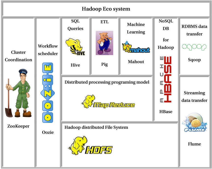
Figure 13-3. The Hadoop ecosystem
Hadoop is a widely used tool. The following are some major companies using Hadoop:
- IBM
- Yahoo
- Amazon
- AOL
- Fox Interactive Media
- New York Times
- Adobe
- eBay
- Ning
The more complete list is available at http://wiki.apache.org/hadoop/PoweredBy.
Up to now, we have discussed some important concepts and tools about big data. As we have done throughout this book, we’ll give an example of big data analytics so you can see big data analytics in action.
Big Data Analytics Example
In this example, we will use data from the Stack Overflow web site (http://stackoverflow.com/). Stack Overflow is a privately held web site that was created in 2008 by Jeff Atwood and Joel Spolsky. The web site serves as a platform for users to ask and answer questions on a wide range of computer programming topics. If you have a specific question about any programing language, you can log in to Stack Overflow and submit your question. You can even tag your questions using keywords such as C++, Java, database, SQL, PHP, and so on. Stack Overflow has a portal where it shares the data. Enthusiastic data scientists can log in and download the data from this portal. We have downloaded a data set from this web site for this big data example.
This example is to understand various concepts related to big data. In this example, we are using a 7GB data set. It’s too small a size for big data, but practical considerations limit us to this size in this example. The following are the steps to be followed in this example:
- Examining the business problem
- Getting the data set
- Starting Hadoop
- Looking at the Hadoop components
- Moving data from the local system to Hadoop
- Viewing the data on HDFS
- Starting Hive
- Creating a table using Hive
- Executing a program using Hive
- Viewing the MapReduce status
- Seeing the final result
Let’s start with the business problem.
Examining the Business Problem
The business wants to extract some basic descriptive statistics such as the total number of questions and the top ten topics from the given file. Data such as the total number of unique users, the top ten users, and the top ten users’ questions is also desired. You could even go to the extent of building a model that detects and suggests the tags automatically when a user enters any question on Stack Overflow web site. For the demo purposes, we only try to find the total number of questions mentioned in the input file.
The data set comes from Stack Overflow. The size of the data set is 7GB, and it’s a text file. This input file needs to be analyzed for finding the basic descriptive statistics.
Starting Hadoop
Hadoop is installed on a Linux machine. In this example, we are using a single-node, or a pseudocluster, Hadoop setup. Basically we are working on one machine only. Since the operating system is Linux, all the operations will be in the form of Linux commands executed in a terminal. The first step is to open a terminal in Linux. The username of our Linux machine is Hadoop. If the username were neo, then you would have neo@local host home. Refer to Figure 13-4.
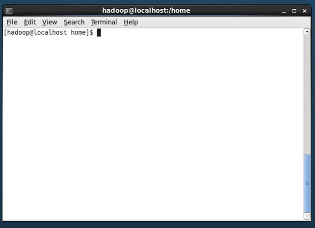
Figure 13-4. Open terminal in Linux
To start Hadoop, you need to go to the Hadoop folder. The path of Hadoop may differ from system to system. Refer to Figure 13-5.
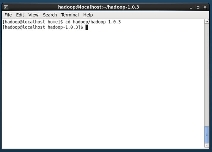
Figure 13-5. The Hadoop folder
Now, you are inside the Hadoop folder. You can start Hadoop, which will start the different components in the ecosystem such as HDFS, the job tracker, the task tracker, and so on. Refer to Figure 13-6.
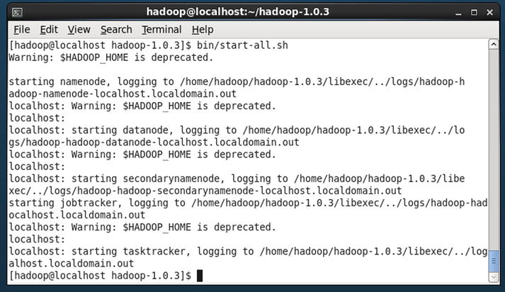
Figure 13-6. Starting Hadoop
start-all.sh is the shell script that will start Hadoop. If you get a warning that Hadoop is deprecated, you can ignore it. The warning will not appear if you are using the latest version of Hadoop. The following are some important messages when you start Hadoop. These messages will give the status of the Hadoop component’s initiation.
- starting namenode, logging to /home/hadoop/hadoop-1.0.3/libexec/../logs/hadoop-hadoop-namenode-localhost.localdomain.out
- starting datanode, logging to /home/hadoop/hadoop-1.0.3/libexec/../logs/hadoop-hadoop-datanode-localhost.localdomain.out
- starting secondarynamenode, logging to /home/hadoop/hadoop-1.0.3/libexec/../logs/hadoop-hadoop-secondarynamenode-localhost.localdomain.out
- starting jobtracker, logging to /home/hadoop/hadoop-1.0.3/libexec/../logs/hadoop-hadoop-jobtracker-localhost.localdomain.out
- localhost: starting tasktracker, logging to /home/hadoop/hadoop-1.0.3/libexec/../logs/hadoop-hadoop-tasktracker-localhost.localdomain.out
Looking at the Hadoop Components
You can now observe that all the Hadoop components have started. You can check on what ports the name node, data, and secondary name node (the backup for the name node) are running. Refer to Figure 13-7. The Jps option shows the ports on which these processes (such as the name node, job tracker, task tracker, and so on) are running.

Figure 13-7. Jps option to see the processes
You can also check and manage Hadoop using the Hadoop administration web interface. To do this, you need to use a web browser and go to http://localhost:50070/dfshealth.jsp. Refer to Figure 13-8.
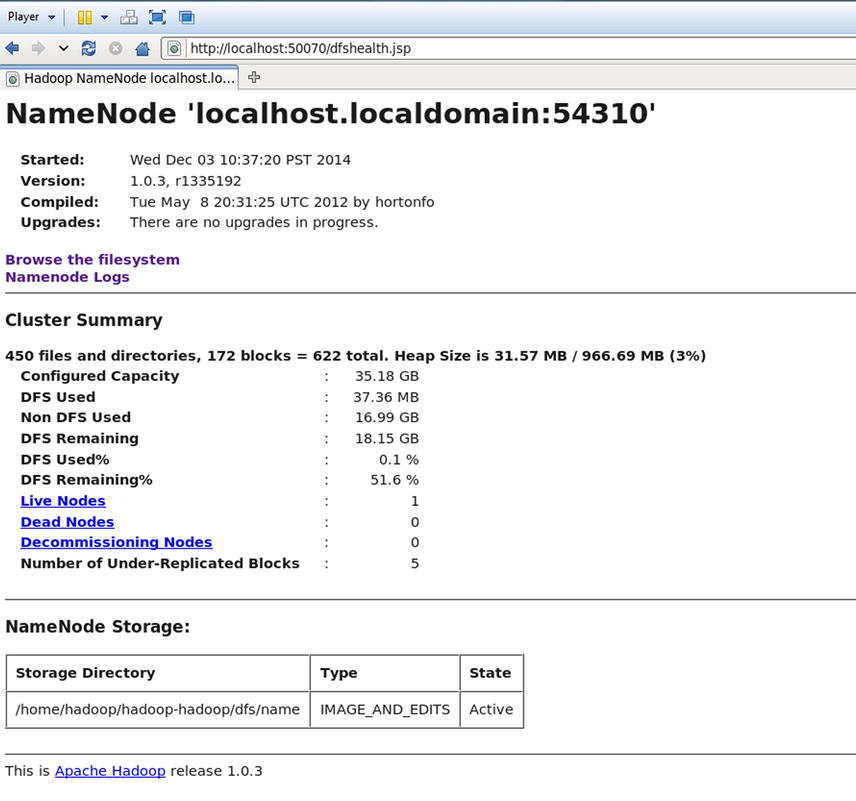
Figure 13-8. Hadoop administration web interface
By clicking the “Browse the filesystem” link in Figure 13-8, you get the file system details shown in Figure 13-9.
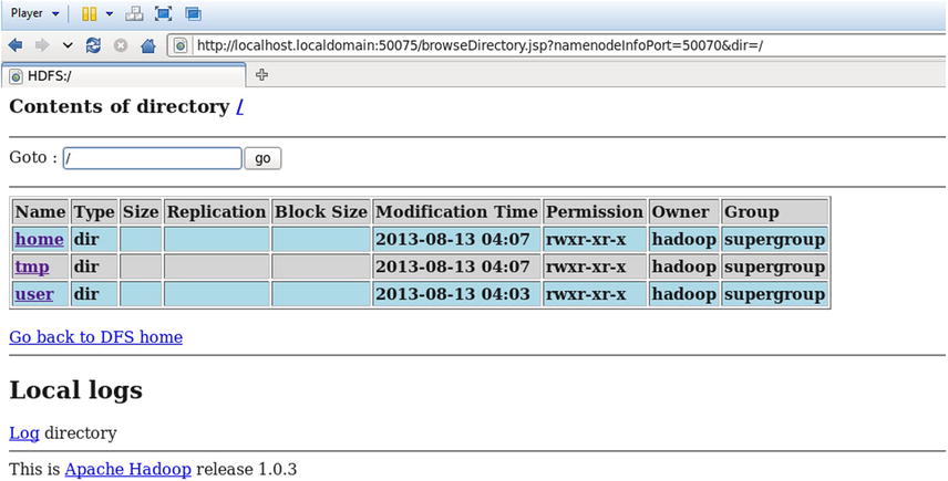
Figure 13-9. The Hadoop distributed file system
The following is the cluster summary (Figure 13-8) before you get the data inside Hadoop:
- 450 files and directories and 171 blocks = 621 total
- Heap size: 31.57MB / 966.69MB (3 percent)
- Configured capacity: 35.18GB
- Distributed file system (DFS) used: 37.36MB
- Non-DFS used: 21.33GB
- DFS remaining: 13.81GB
- DFS used: 0.1 percent
- DFS remaining: 39.27 percent
- Live nodes: 1
- Dead nodes: 0
- Decommissioning nodes: 0
- Number of under-replicated blocks: 5
Moving Data from the Local System to Hadoop
On the DFS file system, you need to move the data file into the HDFS location. The command is simple.
bin/hadoop fs -copyFromLocal /home/final_stack_data.txt stack_data
Type this command and refer to Figure 13-10. This single command will cut the data into many 64MB blocks and distribute them on HDFS.

Figure 13-10. Copying data from the local file system to the Hadoop distributed file system
Viewing the Data on HDFS
Now, as shown in Figure 13-11, the data is successfully loaded on HDFS.
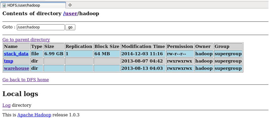
Figure 13-11. Data transferred to HDFS
In Figure 13-11 you can see a new data set named stack_data in HDFS. By clicking it, you can see the content in that data set. Refer to Figure 13-12.
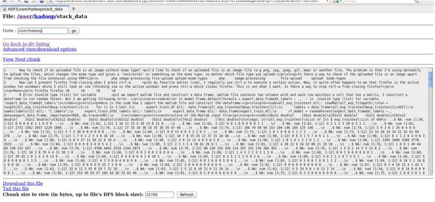
Figure 13-12. Snapshot of a data block
By clicking stack_data, you can see the data in the first chunk, as well as information about other data blocks. Refer to Figure 13-13.

Figure 13-13. Exact location of each data block along with the node IP address
Figure 13-13 shows an important message; because the data set size is 7GB and each block is sized at 64MB, you get a total number of 112 blocks. Each block address is given. Refer to Figure 13-14.

Figure 13-14. Block addresses
Recall that we are not using a multinode cluster. So, you will have only one machine IP address for all the blocks of data. You can see all the blocks are stored at the same IP address (Figure 13-14). If the blocks were stored on different nodes, then you would see different IP addresses for each block. If you click a particular data block, you see its contents. Refer to Figure 13-15.
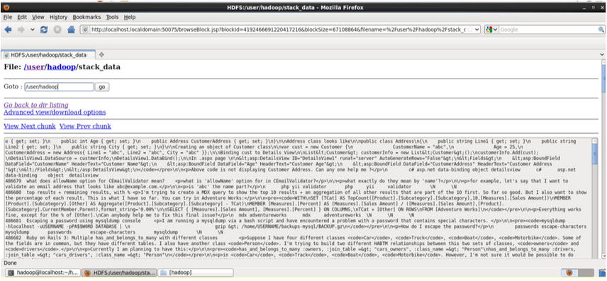
Figure 13-15. Data inside a block
Now that you have the data on a distributed system, you can get started with analytics. As discussed earlier, the task here is to just get some basic descriptive statistics on the data. We used Hive to perform our operations.
Starting Hive
To start Hive, you simply need to type the command hive. Refer to Figure 13-16.
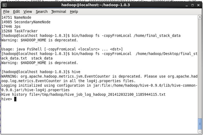
Figure 13-16. Starting Hive
The show tables command will show the existing tables in Hive. The default and previous table names in Hive will appear with this command. Refer to Figure 13-17.
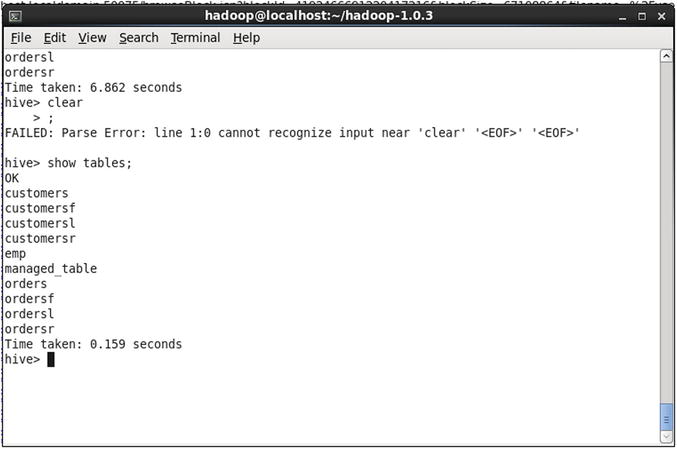
Figure 13-17. Existing tables in Hive
Creating a Table Using Hive
By now you know that Hive is like a SQL engine on top of Hadoop. In the next step, just as you do in SQL, you need to design a table and populate it with data. Refer to Figure 13-18 for the code used to create the table.

Figure 13-18. Creating a table in Hive
Now that the table is created, the following is the command to populate the table with the data on HDFS. Refer to Figure 13-19.
LOAD DATA INPATH '/user/hadoop/stack_over_data' INTO TABLE stack_data_table;

Figure 13-19. Loading the data into a Hive table
Executing a Program Using Hive
You have the table in Hive with the data loaded. Now you need to write the HiveSQL code, and it will automatically get converted into MapReduce code. Refer to Figure 13-20. Execute the following HiveSQL command:
Select count(*) from stack_data_table ;
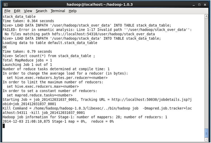
Figure 13-20. Executing the HiveSQL command
Viewing the MapReduce Status
Figure 13-21 shows the status of map and reduce. In this figure, note that the map status is 28 percent and the reduce job is completed by 7 percent.
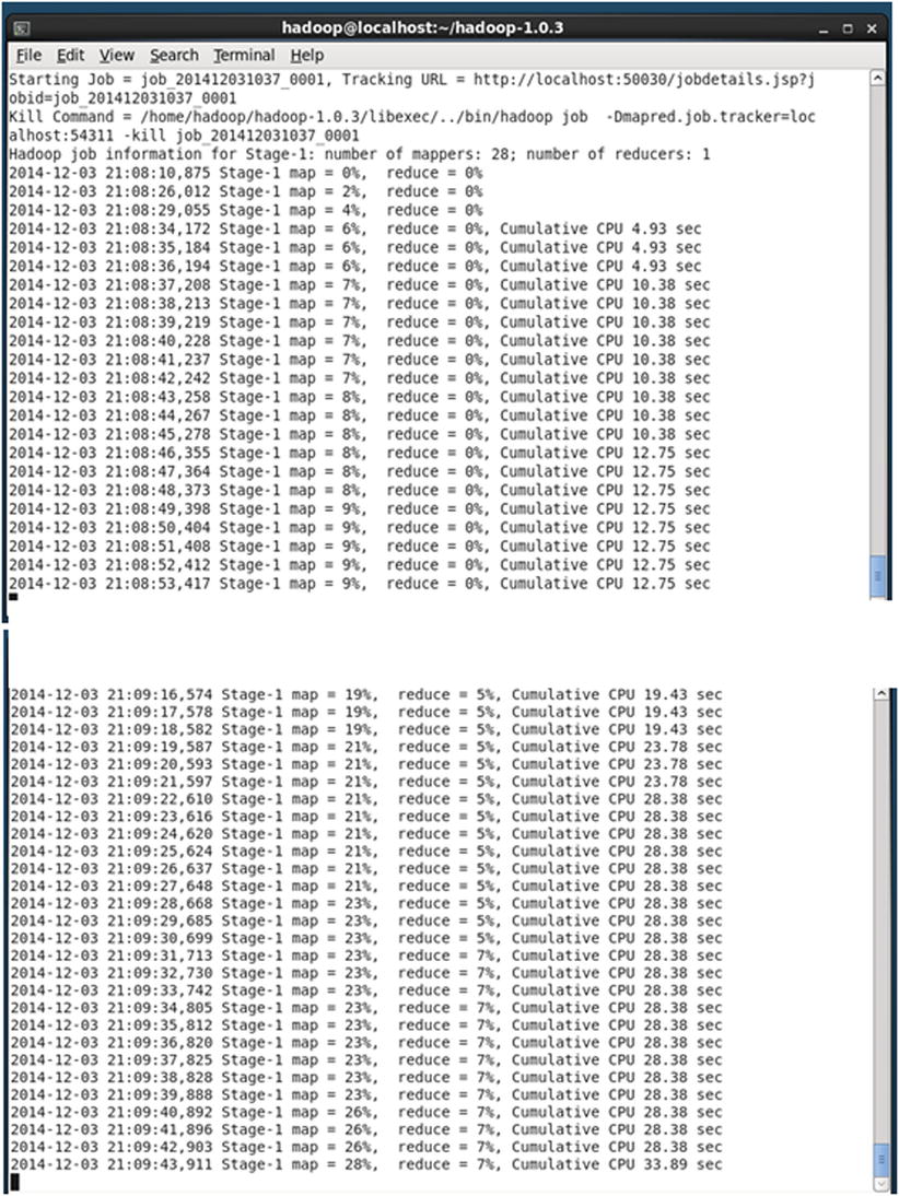
Figure 13-21. The MapReduce intermediate status
Once the MapReduce is completed, you get the results. The total time taken to process this data is about five minutes.
You are simply trying to find the total count of rows, which is the business problem chosen for this demo. When you execute a HiveSQL command, you see that the map and reduce jobs start automatically. The map jobs will be counting rows in each block of data; reduce is for totaling the counts.
The Final Result
The final result shows that there are 6,034,195 records (Figure 13-22). Nearly 6 million questions are included in the original data input file.

Figure 13-22. The final count of rows; the completion of the MapReduce process
Once you understand the basics and see how you got the basic statistics of counting the number of rows, you can write the respective HiveQL commands to get other results such as the top ten topics, the frequency of each topic, and so on.
Conclusion
In this chapter, you learned how a basic big data problem is handled. Big data analytics is the latest buzzword in the market. Big data today is at the beginning stages of its development. A lot of development is expected in this field, particularly in the domains of predictive modeling, text mining, video analytics, and machine learning. As of now, not every algorithm is converted into a MapReduce program. But in the near future, we may have a tool that works on a distributed platform and can perform all the advanced analytics tasks for us. This is a rapidly growing field, so you may see several new tools in the near future. For now, as an exercise, we suggest you do some research on the other components in the Hadoop ecosystem.