
The human brain does a lot of pattern recognition to make sense of raw visual inputs. After the eye focuses on an object, the brain identifies the characteristics of the object—such as its shape, color, or texture—and then compares these to the characteristics of familiar objects to match and recognize the object. In computer vision, that process of deciding what to focus on is called feature detection. A feature in this sense can be formally defined as “one or more measurements of some quantifiable property of an object, computed so that it quantifies some significant characteristics of the object” (Kenneth R. Castleman, Digital Image Processing, Prentice Hall, 1996). An easier way to think of it, though, is that a feature is an “interesting” part of an image. What makes it interesting? Consider a photograph of a red ball on a gray sidewalk. The sidewalk itself probably isn’t that interesting. The ball, however, is probably more interesting, because it is significantly different from the rest of the photograph. Similarly, when a computer analyzes the photograph, the gray pixels representing the sidewalk could be treated as background. The pixels that represent the ball probably convey more information, like how big the ball is or where on the sidewalk it lies.
A good vision system should not waste time—or processing power—analyzing the unimportant or uninteresting parts of an image, so feature detection helps determine which pixels to focus on. This chapter focuses on the most basic types of features: Blobs, Lines, Circles, and Corners. Features represent a new way of thinking about the image—rather than using the image as a whole, focus instead on just a few relevant pieces of an image.
Features also examine an image in a way that may be independent of a single image or other elements of the image. If the detection is robust, a feature is something that could be reliably detected across multiple images. For instance, with the red ball, the features of the ball do not really change based on the location of the ball in the image. The feature detection should work whether the ball is rolling or at rest. The shape and color of the ball should be the same in the lower left corner of the image as it would be in the upper right corner. Similarly, some changes in lighting conditions may change the color of the ball, but in many cases the hue will remain constant. This means that how we describe the feature can also determine the situations in which we can detect the feature.
Our detection criteria for the feature determines whether we can:
Find the features in different locations of the picture (position invariant)
Find the feature if it’s large or small, near or far (scale invariant)
Find the feature if it’s rotated at different orientations (rotation invariant)
In this chapter, we examine the different things we can look for with feature detection, starting with the meat and potatoes of feature detection, the Blob.
Blobs, also called objects or connected components, are regions of similar pixels in an image. This could be a group of brownish pixels together, which might represent food in a pet food detector. It could be a group of shiny metal looking pixels, which on a door detector would represent the door knob. A blob could be a group of matte white pixels, which on a medicine bottle detector could represent the cap. Blobs are valuable in machine vision because many things can be described as an area of a certain color or shade in contrast to a background.
Note
The term background in computer vision can mean any part of the image that is not the object of interest. It may not necessarily describe what is closer or more distant to the camera.
After a blob is identified, we can measure a lot of different things:
A blob’s area tells us how many pixels are in it.
We can measure the dimensions such as width and height.
We can find the center, based on the midpoint or the center of mass (also known as the centroid).
We can count the number of blobs to find different objects.
We can look at the color of blobs.
We can look at its angle to see its rotation.
We can find how close it is to a circle, square, or rectangle—or compare its shape to another blob.
At its most basic, findBlobs()
can be used to find objects that are lightly colored in an image. If no
parameters are specified, the function tries to automatically detect
what is bright and what is dark. The following example looks for
pennies, as shown in Figure 8-1:
from SimpleCV import Image

pennies = Image("pennies.png")

binPen = pennies.binarize()

blobs = binPen.findBlobs()

blobs.show(width=5)
-
Blobs are most easily detected on a binarized image because that creates contrast between the feature in question and the background. This step is not strictly required on all images, but it makes it easier to detect the blobs.
-
Since no arguments are being passed to the
findBlobs()function, it returns aFeatureSetof the continuous light colored regions in the image. We’ll talk about aFeatureSetin more depth in the next chapter, but the general idea is that it is a list of features about the blobs found. AFeatureSetalso has a set of defined methods that are useful when handling features.-
Notice that the
show()function is being called on blobs and not theImageobject. Theshow()function is one of the methods defined with aFeatureSet. It draws each feature in theFeatureSeton top of the original image and then displays the results. By default, it draws the features in green and the function taks acolorandwidthargument to customize the line. For instance, to draw the blobs in red, you could change the above code topacks.show(Color.RED).
The pennies are now green, as is shown in Figure 8-1. After the blob is found, several other functions provide basic information about the feature, such as its size, location, and orientation, as demonstrated in the next block of code:
from SimpleCV import Image

pennies = Image("pennies.png")

binPen = pennies.binarize()

blobs = binPen.findBlobs()

print "Areas: ", blobs.area()

print "Angles: ", blobs.angle()

print "Centers: ", blobs.coordinates() -
The area function returns an array of the area of each feature in pixels. By default, the blobs are sorted by size, so the areas should be ascending in size. The sizes will vary because sometimes it detects the full penny and other times it only detects a portion of the penny.
-
The angle function returns an array of the angles, as measured in degrees, for each feature. The angle is the measure of rotation of the feature away from the x-axis, which is the 0 point. A positive number indicates a counter-clockwise rotation, and a negative number is a clockwise rotation.
-
The coordinates function returns a two-dimensional array of the
(x, y)coordinates for the center of each feature.
These are just a few of the available FeatureSet functions designed to return
various attributes of the features. For information about these
functions, see the FeatureSet section of this chapter.
The findBlobs() function easily
finds lightly colored blobs on a dark background. This is one reason why
binarizing an image makes it easier to detect the object of interest.
But what if the objects of interest are darkly colored on a light
background? In that case, use the invert() function. For instance, the next
example demonstrates how to find the chess pieces in Figure 8-2:

from SimpleCV import Image

img = Image("chessmen.png")

invImg = img.invert()

blobs = invImg.findBlobs()

blobs.show(width=2)

img.addDrawingLayer(invImg.dl())

img.show()
-
The
invert()function turns the black chess pieces white and turns the white background to black.-
The
findBlobs()function can then find the lightly colored blobs as it normally does.-
Show the blobs. Note, however, that this function will show the blobs on the inverted image, not the original image.
-
To make the blobs appear on the original image, take the drawing layer from the inverted image (which is where the blob lines were drawn), and add that layer to the original image.
The result will look like Figure 8-3.

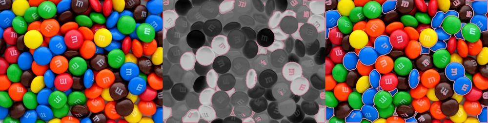
The world does not consist solely of light and dark objects. In many cases, the actual color is more important than the brightness or darkness of the objects. The next example shows how to identify the blue candies in Figure 8-4.

To find the blobs that represent the blue candies, we use the
color information returned from the colorDistance() function that we first
introduced in Chapter 4 and later revisited in
Chapter 5. Here’s the example code:
from SimpleCV import Color, Image

img = Image("mandms.png")

blue_distance = img.colorDistance(Color.BLUE).invert()

blobs = blue_distance.findBlobs()

blobs.draw(color=Color.PUCE, width=3)

blue_distance.show()

img.addDrawingLayer(blue_distance.dl())

img.show()-
The
colorDistance()function returns an image that shows how far away the colors in the original image are from the passed inColor.BLUEargument. To make this even more accurate, we could find the RGB triplet for the actual blue color on the candy, but this works well enough. Because any colors close to blue are black and colors far away from blue are white, we again use theinvert()function to switch the target blue colors to white instead.-
We use the new image to find the blobs representing the blue candies. We can also fine-tune what the
findBlobs()function discovers by passing in a threshold argument. The threshold can either be an integer or an RGB triplet. When a threshold value is passed in, the function changes any pixels that are darker than the threshold value to white and any pixels above the value to black.-
In the previous examples, we have used the
FeatureSetshow()method instead of these two lines (blobs.show()). That would also work here. We’ve broken this out into the two lines here just to show that they are the equivalent of using the other method. To outline the blue candies in a color not otherwise found in candy, they are drawn in puce, which is a reddish color.-
Similar to the previous example, the drawing ends up on the
blue_distanceimage. Copy the drawing layer back to the original image.
The resulting matches for the blue candies will look like Figure 8-5.
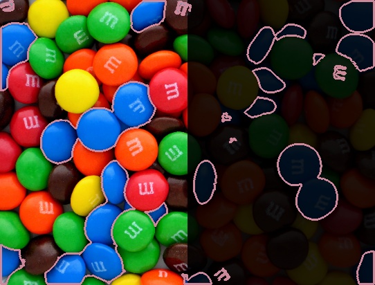
Sometimes the lighting conditions can make color detection more
difficult. To demonstrate the problem, Figure 8-6 is based on the original picture of the
candies, but the left part of the image is darkened. The hueDistance() function is a better choice for
this type of scenario. For instance, if the photo looked like Figure 8-6, where the right half is darkened, then
colorDistance() wouldn't work very
well on the right half. The right half of the image is intentionally
very dark, but the following example shows how the colors can still be
used to find blobs and provide a good example of why hue is more
valuable than RGB color in cases where lighting may vary.

To see how this is a problem, first consider using the previous code on this picture:
from SimpleCV import Color, Image

img = Image("mandms-dark.png")

blue_distance = img.colorDistance(Color.BLUE).invert()

blobs = blue_distance.findBlobs()

blobs.draw(color=Color.PUCE, width=3)

img.addDrawingLayer(blue_distance.dl())

img.show()
The results are shown in Figure 8-7. Notice that only the blue candies on the left are detected.

To resolve this problem use hueDistance() instead of colorDistance(). Because the hue is more
robust to changes in light, the darkened right half of the image won’t
create a problem.
from SimpleCV import Color, Image

img = Image("mandms-dark.png")

blue_distance = img.hueDistance(Color.BLUE).invert()

blobs = blue_distance.findBlobs()

blobs.draw(color=Color.PUCE, width=3)

img.addDrawingLayer(blue_distance.dl())

img.show()-
The one difference in this example is the use of the
hueDistance()function. It works like thecolorDistance()function, but notice that is produces better results, as indicated in Figure 8-8.
A line feature is a straight edge in an image that usually denotes
the boundary of an object. It sounds fairly straightforward, but the
calculations involved for identifying lines can be a bit complex. The
reason is because an edge is really a list of (x, y) coordinates, and any two coordinates
could possibly be connected by a straight line. For instance, Figure 8-9 shows four coordinates and two
different examples of line segments that might connect those four
points. It’s hard to say which one is right—or if either of them are,
since there are also other possible solutions. The way this problem is
handled behind-the-scenes is by using the Hough transform technique.
This technique effectively looks at all of the possible lines for the
points and then figures out which lines show up the most often. The more
frequent a line is, the more likely the line is an actual
feature.

Figure 8-9. Left: Four coordinates; Center: One possible scenario for lines connecting the points; Right: An alternative scenario
To find the line features in an image, use the findLines() function. The function itself
utilizes the Hough transform and returns a FeatureSet of the lines found. The functions
available with a FeatureSet are the
same regardless of the type of feature involved. However, there are
FeatureSet functions that may be
useful when dealing with lines. These functions include:
coordinates()Returns the
(x, y)coordinates of the starting point of the line(s).width()Returns the width of the line, which in this context is the difference between the starting and ending
xcoordinates of the line.height()Returns the height of the line, or the difference between the starting and ending
ycoordinates of the line.length()Returns the length of the line in pixels.
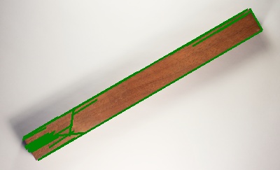
The following code demonstrates how to find and then display the lines in an image. The example looks for lines on a block of wood.
from SimpleCV import Image

img = Image("block.png")

lines = img.findLines()

lines.draw(width=3)

img.show()-
The
findLines()function returns aFeatureSetof the line features.-
This draws the lines in green on the image, with each line having a width of 3 pixels.
The lines found on the image are shown in Figure 8-10.
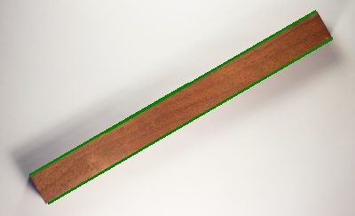
Because this is just a simple block of wood in a well-lit
environment, the findLines() function
does a reasonable job finding the line features using the default values
for its parameters. Many situations may require some tweaking to
findLines() to get the desired
results. For instance, notice that it found the long lines along the top
and bottom of the block, but it did not find the lines along the
side.
The findLines() function
includes five different tuning parameters to help improve the quality of
the results:
- Threshold
This sets how strong the edge should before it is recognized as a line.
- Minlinelength
Sets what the minimum length of recognized lines should be.
- Maxlinegap
Determines how much of a gap will be tolerated in a line.
- Cannyth1
This is a threshold parameter that is used with the edge detection step. It sets what the minimum “edge strength” should be.
- Cannyth2
This is a second parameter for the edge detection which sets the “edge persistence.”
The threshold parameter for findLines() works in much the same way as the
threshold parameter does for the findBlobs() function. If no threshold argument
is provided, the default value it uses is set to 80. Lower threshold
values result in more lines being found by the function; higher values
result in fewer lines being found. Using the block of wood picture
again, here’s the code using a low threshold value:
from SimpleCV import Image

img = Image("block.png")

# Set a low threshold
lines = img.findLines(threshold=10)

lines.draw(width=3)

img.show()
Figure 8-11 shows what the resulting image would look like—with many more lines detected on the block. Notice that it found one of the side lines, but at the cost of several superfluous lines along the grains of wood.

Note
If the threshold value for findLines() is set too high, then no lines
will be found.
One way to get rid of small lines is to use the minlinelength parameter to weed out short
lines. The length of a line is measured in pixels, and the default value
findLines() uses is 30 pixels long.
In the example below, the minimum length is boosted, weeding out some
lines.
from SimpleCV import Image

img = Image("block.png")

lines = img.findLines(threshold=10, minlinelength=50)

lines.draw(width=3)

img.show()
The result is shown in Figure 8-12. Notice that it eliminated a couple of the extra lines, but it came at a cost of eliminating the the side lines again.

Changing the line length doesn’t solve the problem. The two ends
of the image still are not found. In fact, it could create the opposite
problem. Sometimes the algorithm may find very small lines and it needs
to know whether those small line segments actually represent one larger
continuous line. The findLines()
function can ignore small gaps in a line, and recognize it as the larger
overall line. By default, the function combines two segments of a line
if the gap between them is 10 pixels or less. Use the maxlinegap parameter to fine tune how this
works. The following example allows for a larger gap between lines,
potentially allowing it to discover a few small lines that constitute
the edge.
from SimpleCV import Image

img = Image("block.png")

lines = img.findLines(threshold=10, maxlinegap=20)

lines.draw(width=3)

img.show()
The result restores the right edge line again, but once again, it finds a lot of superfluous lines, as demonstrated in Figure 8-13.
While setting the minimum line length decreased the number of
lines found in the painting, adding in a longer gap then dramatically
increased the number of lines. With the bigger gap, the line segments
can be combined to meet the line length requirements and more lines are
then recognized. The last two parameters, cannyth1 and cannyth2, are thresholds for the Canny edge
detector. Roughly speaking, edges are detected by looking for changes in
brightness. The first of these threshold parameters controls how much
the brightness needs to change to detect an edge. The second parameter
controls the threshold for linking together multiple edges. Both of
these parameters act the same way as the previous three parameters:
smaller values mean more lines will be detected, which could just be
adding noise. Conversely, larger values will have less lines detected,
but may mean that some valid lines aren’t being returned. With all of
these parameters, the trick is to work with the parameters until they
are in the range that makes the most sense for the application.
Of course, sometimes it is easier to simply modify the image to reduce the noise rather than fine-tuning the parameters. The following example finds the desired lines on the block:
from SimpleCV import Image

img = Image('block.png')

dist = img.colorDistance((150, 90, 50))

bin = dist.binarize(70).morphClose()

lines = bin.findLines(threshold=10, minlinelength=15)

lines.draw(width=3)

# Move the lines drawn on the binary image back to the main image
img.addDrawingLayer(bin.dl())

img.show()
By binarizing the image, it eliminated a bunch of the noise that was causing the false-positive lines to appear where they should not. As a result, this draws lines around the block, as shown in Figure 8-14.

Circles are the next major feature that the SimpleCV framework can
extract. The method to find circular features is called
findCircle(), and it works the same way
findLines() does. It returns a FeatureSet of the circular features it finds,
and it also has parameters to help set its sensitivity. These parameters
include:
- Canny
This is a threshold parameter for the Canny edge detector. The default value is 100. If this is set to a lower number, it will find a greater number of circles. Higher values instead result in fewer circles.
- Thresh
This is the equivalent of the
thresholdparameter forfindLines(). It sets how strong an edge must be before a circle is recognized. The default value for this parameter is 350.- Distance
Similar to the
maxlinegapparameter forfindLines(). It determines how close circles can be before they are treated as the same circle. If left undefined, the system tries to find the best value, based on the image being analyzed.
As with lines, there are FeatureSet functions that are more appropriate
when dealing with circles, too. These functions include:
radius()As the name implies, this is the radius of the circle.
diameter()The diameter of the circle.
perimeter()This returns the perimeter of the feature, which in the case of a circle, is its circumference. It may seem strange that this isn’t called circumference, but the term perimeter makes more sense when dealing with a non-circular features. Using perimeter here allows for a standardized naming convention.
To showcase how to use the findCircle() function, we’ll take a look at an
image of coffee mugs where one coffee mug also happens to have a
ping-pong ball in it. Because there isn’t any beer in the mugs, we’ll
assume that someone is very good at the game of beer pong—or perhaps is
practicing for a later game? Either way, here’s the example code:
from SimpleCV import Image

img = Image("pong.png")

circles = img.findCircle(canny=200,thresh=250,distance=15)

circles = circles.sortArea()

circles.draw(width=4)

circles[0].draw(color=Color.RED, width=4)

img_with_circles = img.applyLayers()

edges_in_image = img.edges(t2=200)

final = img.sideBySide(edges_in_image.sideBySide(img_with_circles)).scale(0.5)

final.show()
-
Finds the circles in the image. We tested the values for the arguments we’re using here to focus on the circles in which we’re interested.
-
The
sortArea()function is used to sort the circles from the smallest one found to the largest. This lets us identify the circle that is the ping-pong ball, as it will be the smallest circle. It is possible to combine this step with the previous line, too—the result of this would becircles = img.findCircle(canny=200,thresh=250,distance=15).sortArea(). We only separated this into two steps in this example to make it easier to follow.-
This draws all of the circles detected in the green default color. The default line width is a little tough to see, so we’re passing in an argument to increase the width of the line to 4 pixels (see Figure 8-15).
-
This draws a circle in red around the smallest circle, which should be the ping-pong ball.
-
The
draw()function uses a drawing layer for the various circles. This line creates a new image that shows the original image with the drawn circles on top of it.-
In order to show the edges that the
findCircle()function was working with, we use theedges()function to return an image of the edges found in the image. In order for the edges to be the same, we’re passing in the same threshold value (200) toedges()as we did tofindCircle(). Foredges(), this threshold parameter is calledt2, but it’s the same thing as thecannyparameter forfindCircles().-
This combines the various images into a single image. The final result shows the original image, the image of the found edges, and then the original image with the circles drawn on top of it.

The next example combines finding both circle and line features by reading the line on a dial. These types of dials can be found in a variety of places, from large equipment to lighting controls around the house. For our example, we’ll use the dial in Figure 8-16 with four different settings. The code first searches for the dial in the images, and then searches for the line on each dial. Then it measures the angle of that line, and prints it on the image of the dial.

from SimpleCV import Image

# Load the images of four dials with different settings
img0 = Image("dial1.png")
img1 = Image("dial2.png")
img2 = Image("dial3.png")
img3 = Image("dial4.png")

# Store them in an array of images
images = (img0,img1,img2,img3)

# This stores the dial-only part of the images
dials = []

for img in images:
     circles = img.findCircle().sortArea()
     dial = circles[-1].crop()

     lines = dial.findLines(threshold=40,cannyth1=270,cannyth2=400)
     lines = lines.sortLength()
     lines[-1].draw(color=Color.RED)

     lineAngle = lines[-1].angle()

     if (lines[-1].x < (dial.width / 2)):
          if (lines[-1].y < (dial.width / 2)):
                lineAngle = lineAngle - 180
          else:
               lineAngle = 180 + lineAngle

     dial.drawText(str(lineAngle),10,10)
     dial = dial.applyLayers()
     dials.append(dial)

result = dials[0].sideBySide(dials[1].sideBySide(dials[2].sideBySide(dials[3])))
result.show()-
The first step is to find the dial on the image using the
findCircle()function. ThesortArea()function sorts the circles, and because the dial will be the largest circle, we know that it iscircles[-1], the last one in the list.-
Calling the
crop()function on a feature crops the image to just the area of the circle. This then stores the cropped image in thedialvariable.-
Now call the
findLines()function on the cropped image (stored indial).-
The
sortLength()function sorts the list of lines based on their length. Because the dial’s indicator line is most likely the longest line in the image, this will make it easy to identify it in the image.-
The
angle()function computes the angle of a line. This is the angle between the line and a horizontal axis connected at the leftmost point of the line.-
The angles computed in the previous step are correct when the line is on the right side of the dial, but are incorrect for our purposes when on the left side. This is because the angle is calculated from the leftmost point of the line and not the center of the dial. This block of code compensates for this by determining which quadrant the line is in on the left side, and then either adding or subtracting 180 degrees to show the angle as it if were being calculated from the center of the dial instead.
-
After looping through all of the dials, create a single image with the results side by side, as shown in Figure 8-17.

Roughly speaking, corners are places in an image where two lines meet. Corners are interesting in terms of computer vision because corners, unlike edges, are relatively unique and effective for identifying parts of an image. For instance, when trying to analyze a square, a vertical line could represent either the left or right side of the square. Likewise, detecting a horizontal line can indicate either the top or the bottom. On the other hand, each corner is unique. For example, the upper left corner could not be mistaken for the lower right, and vice versa. This makes corners helpful when trying to uniquely identify certain parts of a feature.
The findCorners() function
analyzes an image and returns the locations of all of the corners it can
find. Note that a corner does not need to be a right angle at 90 degrees.
Two intersecting lines at any angle can constitute a corner. As with
findLines() and findCircle(), the findCorners() method returns a FeatureSet of all of the corner features it
finds. While a corner’s FeatureSet
shares the same functions as any other FeatureSet, there are functions that wouldn’t
make much sense in the context of a corner. For example, trying to find
the width, length, or area of a corner doesn’t really make much sense.
Technically, the functions used to find these things will still work, but
what they’ll return are default values and not real data about the
corners.
Similar to the findLines() and
findCircle() functions, findCorners() also has parameters to help
fine-tune the corners that are found in an image. We’ll walk through the
available parameters using an image of a bracket as an example.
from SimpleCV import Image

img = Image('corners.png')

img.findCorners.show()
The little green circles in Figure 8-18
represent the detected corners. Notice that the example finds a lot of
corners. By default, it looks for 50, which is obviously picking up a lot
of false positives. Based on visual inspection, it appears that there are
four main corners. To restrict the number of corners returned, we can use
the maxnum parameter.

from SimpleCV import Image

img = Image('corners.png')

img.findCorners.(maxnum=9).show()
The findCorners() method sorts
all of the corners prior to returning its results, so if it finds more
than the maximum number of corners, it returns only the best ones (see
Figure 8-19). Alternatively, the minquality parameter sets the minimum quality of
a corner before it is shown. This approach filters out the noise without
having to hard code a maximum number of corners for an object.

This is getting better, but the algorithm found two corners in the
lower left and zero in the upper right. The two in the lower left are
really part of the same corner, but the lighting and colors are confusing
the algorithm. To prevent nearby corners from being counted as two
separate corners, set the mindistance
parameter, which sets the minimum number of pixels between two
corners.
from SimpleCV import Image

img = Image('corners.png')

img.findCorners.(maxnum=9, mindistance=10).show()
The results of using a minimum distance are shown in Figure 8-20.

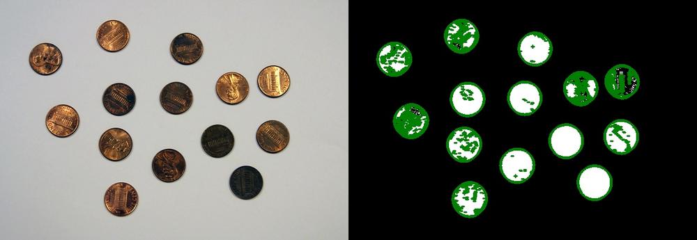
In this example, we take a photo of some coins and calculate what their total value is. To do this, we find the blobs that represent each coin, and then compare them a table of their diameters to look up each coin’s value. In the example, we presume we have a quarter among the coins to act as a reference object. The photo of the coins is shown in Figure 8-21.

from SimpleCV import Image, Blob
import numpy as np

img = Image("coins.png")

coins = img.invert().findBlobs(minsize = 500)

value = 0.0

# The value of the coins in order of their size
# http://www.usmint.gov/about_the_mint/?action=coin_specifications
coin_diameter_values = np.array([
     [ 19.05, 0.10],
     [ 21.21, 0.01],
     [ 17.91, 0.05],
     [ 24.26, 0.25]]);

# Use a quarter to calibrate (in this example we must have one)
px2mm = coin_diameter_values[3,0] /  max([c.radius()*2 for c in coins])

for c in coins:
     diameter_in_mm = c.radius() * 2 * px2mm
     distance = np.abs(diameter_in_mm - coin_diameter_values[:,0])
     index = np.where(distance == np.min(distance))[0][0]
     value += coin_diameter_values[index, 1]

print "The total value of the coins is $", value-
We invert the image to make it easy to find the darker blobs that represent the coins, and eliminate small noisy objects by setting a minimum size.
-
The
coin_diameter_valuesarray represents our knowledge about the relative sizes of the coins versus their values. The first entry in the array is for the smallest coin, a dime. The next largest coin is a penny, then a nickel, and finally a quarter. (This could easily be extended to include half dollars or dollar coins, based on their size.)-
We get a sense of scale by taking the largest diameter in our
FeatureSetand assuming it’s a quarter, similar to the Quarter for Scale example.-
This generates a list of distances that our blob radius is from each coin. Notice that it is slicing the diameter column of the value lookup table.
-
This finds the index of the ideal coin to which the target is closest (minimizing the difference).
-
Add the value from the diameter/value table to our total value.
When running this code using our example photo, the total value of the coins pictured should be $0.91. In this example, the basic detection was fairly straightforward, but we spent most of the time analyzing the data we gathered from the image. In the following chapter, we’ll delve further into these techniques.