One of the most common mistakes of beginning computer vision developers is to overlook lighting and its effect on image quality and algorithm performance. Lighting is a critical component in any vision system and can be the difference between success and failure. After all, without lighting, computer vision would be the study of black rooms with black objects. That would actually make vision programming incredibly easy, but not terribly useful. Instead the lighting should help accomplish three main goals:

Note that in any environment, light radiates from one or more sources and then bounces onto an object (or irradiates it). When filming the object, that surface then radiates the incident light into the camera. It is important to understand this process at an abstract level as it underlies all illumination situations and affects the proposed solutions. A camera does not film the object itself; it films the light reflected from the object (Figure 5-1).

Figure 5-1. Light, camera, action

With lighting, there are three general factors to take into consideration: the source of the light, how the objects being filmed reflect or absorb that light, and how the camera then absorbs and processes the light. It is important to take into account things like the color of the light, the position of the light source in relationship to the target object, and how much of an impact any ambient light might be having on the setup. With the objects, things like the geometry and surface of the object have an impact, as well as its composition and color. If the object’s surface is very reflective, that’s going to require a different lighting setup than an object whose surface absorbs light instead. Finally, with the camera, consider what the camera is capable of, as well as the best settings to use. At the end of the day, if the sensor in the camera can not utilize the light from the light source, then it’s as if the light was not even there in the first place.

If possible, it is easier to control the light sources in the environment than it is to write code to compensate for poor lighting. This first section provides some background on the environment, lighting, and other factors that influence the effectiveness of a vision system. It does not involve much sample code, but understanding the environment makes future coding easier. Of course, in some situations, it is not possible to carefully control the environment. For example, outdoor lighting is heavily subject to the weather and time of day. Given these challenges, the next section of this chapter covers how to use the SimpleCV framework to compensate for different lighting situations. But first, some background on creating an environment conducive to machine vision.

Ideally, within the environment, create a situation where the lighting is as consistent and controlled as possible. If there is a lot of light contamination from external light sources, it may help to create an enclosure to block that light. Alternatively, some sources of light can be controlled with filters on the camera. It is even important to consider how the objects themselves will be presented to the camera. Will they be in a consistent location? If they’re not going to be in the same location, then a spotlight probably is not the best lighting choice. Will the objects be moving? If they are moving—such as on a conveyor belt—a strobe light might may help to capture the most relevant information. Sometimes a new light source can be added or the light source’s orientation can be changed to improve the quality of the image captured. Any changes made to the environment to increase the consistency when filming one object to the next will make the programming easier.

Light and Color

The color of a light source is another important consideration when selecting a lighting source. Scientifically speaking, visible light is the part of the electromagnetic spectrum that ranges from low frequency (long wavelength) red light to high frequency (short wavelength) violet light. We use the term visible light to talk about the range of the spectrum that humans can see. Different illumination systems generate different colors of light. For example, sunlight at noon is different than a white LED light, which is different than the light of a laser pointer pen. When comparing sources, it is often useful to draw a graph with the rainbow of colors on the x-axis and the amount of light at each color plotted on the y-axis (see Figure 5-2 for an example).

Figure 5-2. Histogram superimposed on the visible light spectrum

One reason that the color of the light is important is that different surfaces respond differently to various colors of light. One example of this effect is an ordinary white t-shirt. When viewing a white t-shirt under most lighting conditions, it appears more or less white. When using a black light, the same shirt can appear to be glowing violet. For any situation where an objects is illuminated by light (regardless of its source), this same effect is in play. This effect can have a significant impact when using color to identify objects and segment images. You can see the impact from different colored light sources in Figure 5-3. If the wrong color light changes the apparent color of the image, the code will fail.

Figure 5-3. Using different colored lights creates different contrasts

Sometimes the color balance of a picture is a bit off, requiring some degree of correction. This is done with a ColorCurve object. The color is most simply thought of as a graph where the x-axis is the intensity of the color in the original image and the y-axis is the new intensity. For example, if the curve for the red channel goes through the point (100, 120), then any pixel that had a red value of 100 in the original image will have a value of 120 in the new image. Obviously defining these new values for all 256 possible red values, plus all 256 green values, plus all 256 possible blue values would be a time consuming mess. Instead, ColorCurves are defined with several points, and the rest are interpolated. For example, a curve for the red channel defined by the points (0, 0), (128, 128), and (256, 128) will leave all the low and middle intensity reds untouched, but it will reduce the high intensity reds.

To apply a color curve, first create the ColorCurve for each color channel. When working with RGB color, the result is then applied with the applyRGBCurve() function. The function takes three arguments: a curve for the R channel, a curve for the G channel, and a curve for the B channel. Curves can also be applied to HSV images with the applyHSVCurve() function. It once again takes three arguments of the three curves representing the H, S, and V channels.

The following example demonstrates how to use color curves to apply an old-time photo effect to images from the webcam.

from SimpleCV import Camera, Display, ColorCurve, Image

screenSize = (640, 480)

rCurve = ColorCurve([[0,0],[64,64],[128,128],[256,128]])  

gbCurve = ColorCurve([[0,16],[64,72],[128,148],[256,256]])  

cam = Camera(-1, {'width': screenSize[0], 'height': screenSize[1]} )

disp = Display(screenSize)

while not disp.isDone():
     img = cam.getImage()

     coloredImg = img.applyRGBCurve(rCurve, gbCurve, gbCurve)  

     erodedImg = coloredImg.erode(1)  

     erodedImg.save(disp)

The first curve will be used for the red channel. It reduces the high intensity red colors.

The second curve will be used for the green and blue channels. It provides a slight boost to the mid-level green and blue channels.

Apply the curve to the image. Note that rCurve is used for just the red channel, whereas gbCurve is passed both for the green and blue channels.

Adding an erode to the image provides a little additional old-time photo look to the image.

The Target Object

While the brightness and color refer to the light source, the nature of the object itself also affects how light interacts with it. When light reflects off of an object, it always follows the law of reflection, which states that the angle at which the light approached the object (the incident ray) is the same angle at which the light will leave the object (the reflected ray). When an object’s surface is completely smooth, as in the case of a mirror, then all of the incoming light will be reflected uniformly away from the object. This is known as a specular reflection and will make the object seem shiny because of all of the reflected light. However, if the surface of the object is not smooth, such as with a piece of paper, then the incoming light hits the varied surface at different angles—and because it still obeys the law of reflection, the reflected light then leaves the object using those same angles. Because the light rays are not leaving the object in a uniform manner, the light is scattered and the object appears to have more of a dull finish. This is known as a diffused reflection (see Figure 5-4).

Figure 5-4. How a rough surface diffuses light

The nature of an object, or what it consists of, impacts more then just how smooth its surface is. Some materials absorb light; some transmit the light and let it shine right through. Some materials are fluorescent and when they absorb light at one wavelength, may emit light at a different wavelength. Then there’s also the geometry of the object; a curved surface is going to reflect light differently than a flat one. One of the easiest ways to deal with all of these considerations is a simple trial and error process to test how various light sources interact with a sample object. Because the lighting can have such a dramatic impact on the image quality, it’s a good idea to do this early in the process of developing a vision system.

The following terms are sometimes used when describing the surface of an object:

Lambertian

Normal or matte surfaces. Light reflects predictably off the object, based only on the position of the light source. Examples include terra cotta, unfinished wood, paper, and fabric. These types of objects are among the easiest to capture with computer vision and are the most robust under different lighting considerations. An example image is shown in Figure 5-5.

Sub-surface scattering

Light penetrates the objects, interacts with the material, and exits at another point. Examples include milk, skin, bone, shells, wax, and marble. The position of the source of light can sometimes have unpredictable results, making it important to plan lighting carefully and have consistent lighting to ensure high quality results. An example is shown in Figure 5-6.

Specular

Shiny objects, such as polished metals, glass, and mirrors. These objects are difficult to use in computer vision systems because their surfaces may include reflections on other objects from their surroundings. When dealing with smooth specular surfaces, it is common to have lighting in a specific pattern and analyze the reflection, rather than the object itself. An example is demonstrated in Figure 5-7.

Figure 5-5. The Terracotta Army, a lambertian surface

Figure 5-6. Sub-surface scattering through wax

Figure 5-7. A glass sculpture with a specular surface

Albedo

A measure of of the percentage of light reflected by an object. Albedo is measured from zero to one, with one meaning that 100% of the light directed on to the object is then reflected. Objects with a higher albedo look more white. Objects with a lower albedo appear darker, as they absorb most of the light that hits them. This determines the quantity of light that usable in an application. An example is shown in Figure 5-8.

Figure 5-8. The albedo effect

Besides strength and color, light is also classified according to point-source, diffuse, and ambient light. A point source light is basically a light bulb or the sun. A diffuse source is light that has been diffused though another object, such as clouds or a diffuser attached to a camera flash. Ambient lighting is a catch-all term for light that has bounced off multiple objects before the object of interest.

Lighting Techniques

The final area to consider is the lighting techniques. The following is a quick outline of some of the more popular techniques:

Technique	Lighting Type & Direction	Advantages	Disadvantages	Example
Diffuse Dome Lighting	Diffused light source, placed in front of the object	Effective at lighting curved, specular surfaces	Usually requires close proximity to the object
Diffuse On Axis Lighting	Diffused light source, placed in front of the object	Effective at lighting flat, specular surfaces	Usually requires close proximity to the object
Bright Field Lighting	A point light source, placed in front of the object	The most commonly used lighting technique. It’s good for enhancing topographical details.	With specular or curved surfaces, it can create strong reflections
Dark Field Lighting	A point light source, placed at the side of the object	Good for finding surface imperfections	Does not illuminate flat, smooth surfaces
Diffuse Backlighting	A diffuse light source, placed behind the object	Creates a high-contrast silhouette of an object; useful for finding the presence of holes or gaps	The edges of the silhouette may be fuzzy
Collimated Backlighting	A point light source, placed behind the object	Creates sharp edges on a silhouette, so good for measuring the overall dimensions of an object	Not good for recording topographical details

In addition to the illumination, it is also important to understand the color of the image. Although color sounds like a relatively straightforward concept, different representations of color are useful in different contexts. The following examples work with an image of The Starry Night by Vincent van Gogh, as shown in Figure 5-9.

Figure 5-9. The Starry Night, used in the examples that follow

In the SimpleCV framework, the colors of an individual pixel are extracted with the getPixel() function. This was previously demonstrated in Chapter 4.

from SimpleCV import Image

img = Image('starry_night.png')

print img.getPixel(0, 0)  

One criticism of RGB is that it does not specifically model luminance. Yet the luminance/brightness is one of the most common properties to manipulate. In theory, the luminance is the relationship of the of R, G, and B values. In practice, however, it is sometimes more convenient to separate the color values from the luminance values. For example, the difference between a bright yellow and a dark yellow is non-intuitively controlled by the amount of blue. The solution is HSV, which stands for hue, saturation, and value. The color is defined according to the hue and saturation, while value is the measure of the luminance/brightness. The HSV color space is essentially just a transformation of the RGB color space because all colors in the RGB space have a corresponding unique color in the HSV space, and vice versa. It is easy to convert images between the RGB and HSV color spaces, as is demonstrated below.

from SimpleCV import Image

img = Image('starry_night.png')

hsv = img.toHSV()  

print hsv.getPixel(25,25)  

rgb = hsv.toRGB()  

print rgb.getPixel(25,25)  

The HSV color space is particularly useful when dealing with an object that has a lot of specular highlights or reflections. In the HSV color space, specular reflections will have a high luminance value (V) and a lower saturation (S) component. The hue (H) component may get noisy depending on how bright the reflection is, but an object of solid color will have largely the same hue even under variable lighting. We’ll look at hue segmentation further in Chapter 8.

Grayscale is the final color encoding scheme commonly used in programs developed with the SimpleCV framework. A grayscale image represents the luminance of the image, but lacks any color components. It is often referred to as a black-and-white image, though it is important to understand the difference between a grayscale and a binary black-and-white image. In the later case, there are only two values: 0 and 1 for pure black and pure white, respectively. In contrast, an 8-bit grayscale image has many shades of grey, usually on a scale from 0 to 255. The challenge is to create a single value from 0 to 255 out of the three values of red, green, and blue found in an RGB image. There is no single scheme for doing this, but it is done by taking a weighted average of the three. To create a grayscale image:

from SimpleCV import Image

img = Image('starry_night.png')

gray = img.grayscale()  

print gray.getPixel(0,0) 

Notice that it returns the same number three times. This keeps a consistent format with RGB and HSV, which both return three values. However, since grayscale only has one value, representing the luminance, the same value is repeated three times. To get the grayscale value for a particular pixel without having to convert the image to grayscale, use getGrayPixel().

Figure 5-10. The Starry Night, converted to grayscale

Chapter 3 introduced the concept of segmentation, which is the process of dividing an image into areas of related content. These areas consist of pixels that all share a particular characteristic, and one of the more frequently used characteristics is color. It is easy to use color to segment an image. This technique is very effective when a color of the desired object is substantially different from the background color, such as tracking a brightly colored object such as a ball. In this case, use the color difference to segment the image and remove the background from the image, leaving just the object of interest.

This works by essentially subtracting one image from another. To understand this, first consider how subtraction works with pixels (a topic which is covered more extensively in the next chapter). Assume that the pixel at point (0, 0) is purple, with the RGB triplet (100, 0, 100). Take an identical pixel—(100, 0, 100)—and subtract it from the original pixel. To do this, simply subtract each element from its corresponding value. (100, 0, 100) - (100, 0, 100) = (0, 0, 0). Since (0, 0, 0) is the RGB value for black, subtracting the same RGB value from a pixel results in a black pixel. Different colored pixels can also be subtracted from each other. For example, (100, 0, 100) - (90, 0, 10) = (10, 0, 90), which results in a mostly blue pixel. Subtracting images is just like subtracting pixels, with the system going through the image on a pixel-by-pixel basis and performing the subtraction for each pixel.

Color segmentation is based on subtracting away the pixels that are far away from the target color, while preserving the pixels that are similar to the color. This requires measuring all of the colors involved to gauge how far away they are from the target color. The Image class has a function called colorDistance() that computes the distance between every pixel in an image and a given color. This function takes as an argument the RGB value of the target color, and it returns another image representing the distance from the specified color. This is perhaps easier to understand by looking at an example, so let’s work with a picture of a yellow glue gun, as seen in Figure 5-11.

Figure 5-11. A yellow glue gun

from SimpleCV import Image, Color

yellowTool = Image("yellowtool.png")

yellowDist = yellowTool.colorDistance((223, 191, 29))  

yellowDistBin = yellowDist.binarize(50).invert()  

yellowDistBin.show()

The resulting image should look like Figure 5-12.

Figure 5-12. The yellow color distance

Now the distance image can be subtracted from the original image to remove any portions of the image that are not yellow.

from SimpleCV import Image, Color

yellowTool = Image("yellowtool.png")

yellowDist = yellowTool.colorDistance((223, 191, 29))

yellowDistBin = yellowDist.binarize(50).invert()

onlyYellow = yellowTool - yellowDistBin

onlyYellow.show()

This will result in an image with only the yellow body of the tool and everything else blacked out, as shown in Figure 5-13.

Figure 5-13. Only the yellow body of the tool remains

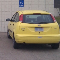
Let’s walk through an example where we detect if a car is illegally parked in a handicap parking space. At the Sight Machine offices, there is a repeat offender who drives a yellow car, parks illegally, and does not have a handicap sticker. Figure 5-14 shows what the image looks like without the car in the spot.

Figure 5-14. The parking lot at the Sight Machine offices

Figure 5-15 shows the offending car in the handicap parking spot.

Figure 5-15. The offending car parked illegally in the handicap parking spot

A simple test would be to simply look for yellow in the image. However, if the yellow car is parked adjacent to the handicap spot, then there is no violation. Instead, this “yellow detector” vision system will have to look whether yellow appears in a particular area in the image.

First, load the images of the car:

from SimpleCV import Image

car_in_lot = Image("parking-car.png")  

car_not_in_lot = Image("parking-no-car.png")  

The next step is to use the picture of the car in the spot to determine the area to inspect. Since the original image contains both acceptable and illegal parking spaces, it needs to be cropped to cover only the handicap space. The whole image is 800×600 pixels. The location of the handicap space is the box around the car, sometimes referred to as the Region of Interest (ROI). In this case, the ROI starts at (470, 200) and is about 200×200 pixels.

from SimpleCV import Image

car_in_lot = Image("parking-car.png")

car_not_in_lot = Image("parking-no-car.png")

car = car_in_lot.crop(470,200,200,200)  

# Show the results
car.show()

The resulting picture should look like Figure 5-16.

Figure 5-16. The cropped image

Now that the image is narrowed down to only the handicap spot, the next step is to find the car in the image. The general approach is similar to the yellow glue gun example given earlier. First, find the pixels that are near yellow:

from SimpleCV import Image

car_in_lot = Image("parking-car.png")

car_not_in_lot = Image("parking-no-car.png")

car = car_in_lot.crop(470,200,200,200)

yellow_car = car.colorDistance(Color.YELLOW)  

# Show the results
yellow_car.show()

The resulting image should look like Figure 5-17.

Figure 5-17. The color distances away from yellow

With the color distances computed, subtract out the other colors, leaving only yellow components. This should result in just the car, subtracting out the rest of the image.

from SimpleCV import Image

car_in_lot = Image("parking-car.png")

car_not_in_lot = Image("parking-no-car.png")

car = car_in_lot.crop(470,200,200,200)

yellow_car = car.colorDistance(Color.YELLOW)

only_car = car - yellow_car  

# Show the results
only_car.show()

As expected, only the car remains, as shown in Figure 5-18.

Figure 5-18. The yellow of the car

To compare this to images that do not have the yellow car in them, there must be some sort of metric to represent the car. One simple way to do this is with the meanColor() function. As the name implies, this computes the average color for the image:

from SimpleCV import Image

car_in_lot = Image("parking-car.png")

car_not_in_lot = Image("parking-no-car.png")

car = car_in_lot.crop(470,200,200,200)

yellow_car = car.colorDistance(Color.YELLOW)

only_car = car - yellow_car

print only_car.meanColor()  

This is the metric for the space when occupied by the yellow car. Repeat the process for the empty place.

from SimpleCV import Image

car_in_lot = Image("parking-car.png")

car_not_in_lot = Image("parking-no-car.png")

car = car_in_lot.crop(470,200,200,200)

yellow_car = car.colorDistance(Color.YELLOW)

only_car = car - yellow_car

no_car = car_not_in_lot.crop(470,200,200,200)

without_yellow_car = no_car.colorDistance(Color.YELLOW)  

# Show the results
without_yellow_car.show()

Notice in Figure 5-19 that this essentially creates an “empty” image.

Figure 5-19. The color distance away from yellow when the car is not present

Once again, subtract the color distance image and compute the mean color:

from SimpleCV import Image

car_in_lot = Image("parking-car.png")

car_not_in_lot = Image("parking-no-car.png")

car = car_in_lot.crop(470,200,200,200)

yellow_car = car.colorDistance(Color.YELLOW)

only_car = car - yellow_car

no_car = car_not_in_lot.crop(470,200,200,200)

without_yellow_car = no_car.colorDistance(Color.YELLOW)

only_space = no_car - without_yellow_car

print only_space.meanColor()

The resulting mean color will be: (5.031350000000001, 3.6336250000000003, 4.683625). This contrasts substantially with the mean color when the car is in the image, which was (25.604575, 18.880775, 4.4940750000000005). The amount of blue is similar, but there is substantially more red and green when the car is in the image. This should sound right given that yellow is created by combining red and green.

Given this information, it should be relatively easy to define the thresholds for determining if the car is in the lot. For example, something like the following should do the trick:

from SimpleCV import Image

car_in_lot = Image("parking-car.png")

car_not_in_lot = Image("parking-no-car.png")

car = car_in_lot.crop(470,200,200,200)

yellow_car = car.colorDistance(Color.YELLOW)

only_car = car - yellow_car

(r, g, b) = only_car.meanColor()

if ((r > 15) and (g > 10):  
     print "The car is in the lot.  Call the attendant."

In cases where there is enough yellow—as defined by enough red and green—it indicates that the violating car is in the lot. If not, it does nothing. Note that this prints the message for any yellow car in the parking space, as well as any other large, yellow object. Of course this is just a basic example, it could be refined by matching other objects of the car, such as its shape or size.