3 Advanced concepts of differential privacy for machine learning

This chapter covers

• Design principles of differentially private machine learning algorithms
• Designing and implementing differentially private supervised learning algorithms
• Designing and implementing differentially private unsupervised learning algorithms
• Walking through designing and analyzing a differentially private machine learning algorithm

In the previous chapter we investigated the definition and general use of differential privacy (DP) and the properties of differential privacy that work under different scenarios (the postprocessing property, group property, and composition properties). We also looked into common and widely adopted DP mechanisms that have served as essential building blocks in various privacy-preserving algorithms and applications. This chapter will walk through how you can use those building blocks to design and implement multiple differentially private ML algorithms and how you can apply such algorithms in real-world scenarios.

3.1 Applying differential privacy in machine learning

In chapter 2 we investigated different DP mechanisms and their properties. This chapter will showcase how you can use those DP mechanisms to design and implement various differentially private ML algorithms.

As shown in figure 3.1, we are considering a two-party ML training scenario with a data owner and a data user. The data owner provides the private data, which is the input or the training data. Usually, the training data will go through a data preprocessing stage to clean the data and remove any noise. The data user will then perform a specific ML algorithm (regression, classification, clustering, etc.) on this personal data to train and produce an ML model, which is the output.

Figure 3.1 The design principles of differentially private ML

As we all know, DP has received growing attention over the last decade. As a result, various differentially private ML algorithms have been proposed, designed, and implemented by both industrial and academic researchers. DP can be applied to prevent data users from inferencing the private data by analyzing the ML model. As depicted in figure 3.1, the perturbation can be applied at different steps in the ML process to provide DP guarantees. For instance, the input perturbation approach adds noise directly to the clean private data or during the data preprocessing stage. The algorithm perturbation approach adds noise during the training of ML models. The objective perturbation approach adds noise to the objective loss functions of the ML model. Finally, output perturbation adds noise directly to the trained ML model that is the output of the ML algorithms.

Figure 3.2 identifies a set of popular perturbation strategies applied in ML algorithms as examples presented in this chapter. Of course, there are other possible examples out there, but we will stick to these methods, and we will discuss these perturbation approaches in detail in the next section.

Figure 3.2 DP perturbation strategies and the sections they’re discussed in

Let’s walk through these four common design principles for differentially private ML algorithms, starting with input perturbation.

3.1.1 Input perturbation

In input perturbation, noise is added directly to the input data (the training data), as shown in figure 3.3. After the desired non-private ML algorithm computation (the ML training procedure) is performed on the sanitized data, the output (the ML model) will be differentially private. For example, consider the principal component analysis (PCA) ML algorithm. Its input is the covariance matrix of the private data, and its output is a projection matrix (the output model of PCA). Before performing the Eigen-decomposition on the covariance matrix (the input), we can add a symmetric Gaussian noise matrix to the covariance matrix [1]. Now the output will be a differentially private projection matrix (remember, the goal here is not releasing the projected data but the DP-projection matrix).

Figure 3.3 How input perturbation works

Input perturbation is easy to implement and can be used to produce a sanitized dataset that can be applied to different kinds of ML algorithms. Since this approach focuses on perturbing the input data to ML models, the same procedure can be generalized to many different ML algorithms. For instance, the perturbed covariance matrix can also be the input for many different component analysis algorithms, such as PCA, linear discriminant analysis (LDA), and multiple discriminant analysis (MDA). In addition, most DP mechanisms can be utilized in input perturbation approaches, depending on the properties of the input data.

However, input perturbation usually requires adding more noise to the ML input data, since the raw input data usually has a higher sensitivity. As discussed in chapter 2, sensitivity in DP is the largest possible difference that one individual’s private information could make. Data with a higher sensitivity requires us to add more noise to provide the same level of privacy guarantee. In section 3.2.3, we’ll discuss differentially private linear regression to show you how input perturbation can be utilized when designing DP ML algorithms.

3.1.2 Algorithm perturbation

With algorithm perturbation, the private data is input to the ML algorithm (possibly after non-private data preprocessing procedures), and then DP mechanisms are employed to generate the corresponding sanitized models (see figure 3.4). For ML algorithms that need several iterations or multiple steps, DP mechanisms can be used to perturb the intermediate values (i.e., the model parameters) in each iteration or step. For instance, Eigen-decomposition for PCA can be performed using the power iteration method, which is an iterative algorithm. In the noisy power method, Gaussian noise can be added in each iteration of the algorithm, which operates on the non-perturbed covariance matrix (i.e., the input), leading to DP PCA [2]. Similarly, Abadi proposed a DP deep learning system that modifies the stochastic gradient descent algorithm to have Gaussian noise added in each of its iterations [3].

Figure 3.4 How algorithm perturbation works: Input is private data. Then we preprocess the data (non-private). Next, we perturb the intermediate values during training iterations inside the ML algorithm. Finally, we have a DP ML model.

As you can see, algorithm perturbation approaches are usually applied to ML models that need several iterations or multiple steps, such as linear regression, logistic regression, and deep neural networks. Compared with input perturbation, algorithm perturbation requires a specific design for different ML algorithms. However, it usually introduces less noise while using the same DP privacy budget, since the intermediate values in the training ML models generally have less sensitivity than the raw input data. Less noise usually leads to better utility of the DP ML models. In section 3.3.1 we’ll introduce differentially private k-means clustering to discuss further how to utilize algorithm perturbation in the design of DP ML.

3.1.3 Output perturbation

With output perturbation we use a non-private learning algorithm and then add noise to the generated model, as depicted in figure 3.5. For instance, we could achieve DP PCA by sanitizing the projection matrix produced by the PCA algorithm by using an exponential mechanism (i.e., by sampling a random k-dimensional subspace that approximates the top k PCA subspace).

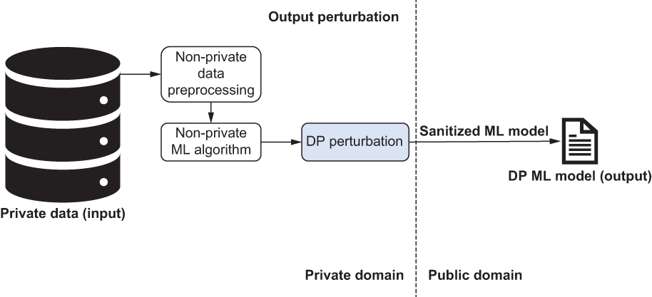
Figure 3.5 How output perturbation works: Input is private data. Then we preprocess the data (non-private). Next, we apply DP perturbation to the non-private ML algorithm. Finally, we have a DP ML model.

In general, output perturbation approaches are usually applied to ML algorithms that produce complex statistics as their ML models. For example, feature extraction and dimensionality reduction algorithms typically publish the extracted features. Thus, using a projection matrix for dimensionality reduction is a suitable scenario for using output perturbation. However, many supervised ML algorithms that require releasing the model and interacting with the testing data multiple times, such as linear regression, logistic regression, and support vector machines, are not suitable for output perturbation. In section 3.2.1 we’ll walk through differentially private naive Bayes classification to discuss further how we can utilize output perturbation in DP ML.

3.1.4 Objective perturbation

As shown in figure 3.6, objective perturbation entails adding noise to the objective function for learning algorithms, such as empirical risk minimization, that use the minimum/maximum of the noisy function as the output model. The core idea of empirical risk minimization is that we cannot know exactly how well an algorithm will work with actual data because we don’t know the true distribution of the data that the algorithm will work on. However, we can measure its performance on a known set of training data, and we call this measurement the empirical risk. As such, in objective perturbation, a vector mechanism can be designed to accommodate noise addition. To learn more about exactly how to do that, refer to section A.2.

Figure 3.6 How objective perturbation works: The input is private data. Then we preprocess the data (non-private). Next, we perturb the objective function of the ML model during the training. Finally, we have a DP ML model.

As you’ll know, a sample space is the set of all possible outcomes of an event or experiment. A real-world sample space can sometimes include both bounded values (values that lie within a specific range) and unbounded values covering an infinite set of possible outcomes. However, most perturbation mechanisms assume a bounded sample space. When the sample space is unbounded, it leads to unbounded sensitivity, resulting in unbounded noise addition. Hence, if the sample space is unbounded, we can assume that the value of each sample will be truncated in the preprocessing stage, and the truncation rule is independent of the private data. For instance, we could use common knowledge or extra domain knowledge to decide on the truncation rule. In section 3.2.2 we’ll discuss differentially private logistic regression and objective perturbation in DP ML.

3.2 Differentially private supervised learning algorithms

Supervised learning employs labeled data where each feature vector is associated with an output value that might be a class label (classification) or a continuous value (regression). The labeled data is used to build models that can predict the labels of new feature vectors (during the testing phase). With classification, the samples usually belong to two or more classes, and the objective of the ML algorithm is to determine which class the new sample belongs to. Some algorithms might achieve that by finding a separating hyperplane between the different classes. An example application is face recognition, where a face image can be tested to ascertain that it belongs to a particular person.

Multiple classification algorithms can be used for each of the previously mentioned applications, such as support vector machines (SVMs), neural networks, or logistic regression. When a sample label is a continuous value (also referred to as a dependent or response variable) rather than a discrete one, the task is called regression. The samples are formed of features that are also called independent variables. The target of regression is fitting a predictive model (such as a line) to an observed dataset such that the distances between the observed data points and the line are minimized. An example of this would be estimating the price of a house based on its location, zip code, and number of rooms.

In the following subsections, we’ll formulate the DP design of the three most common supervised learning algorithms: naive Bayes classification, logistic regression, and linear regression.

3.2.1 Differentially private naive Bayes classification

First, let’s look into how differentially private naive Bayes classification works, along with some mathematical explanations.

Naive Bayes classification

In probability theory, Bayes’ theorem describes the probability of an event based on prior knowledge of conditions that might be related to the event. It is stated as follows:

• A and B are the events.

• P(A|B) is the probability of A, given B is true.

• P(B|A) is the probability of B, given A is true.

• P(A) and P(B) are the independent probabilities of A and B.

The naive Bayes classification technique uses Bayes’ theorem and the assumption of independence between every pair of features.

First, let the instance to be classified be the n -dimensional vector X = [x₁, x₂,...,x_n], the names of the features be [F₁, F₂,...,F_n], and the possible classes that can be assigned to the instance be C = [c₁, c₂,...,c_n].

The naive Bayes classifier assigns the instance X to the class F_S if and only if P(C_s|X) P(C_j|X) for 1 ≤ j ≤ k and j ≠ s. Hence, the classifier needs to compute P(C_j│X) for all classes and compare these probabilities.

We know that when using Bayes’ theorem, the probability P(C_j│X) can be calculated as

Since P(X) is the same for all classes, it is sufficient to find the class with the maximum P(X|C_j) ∙ P(C_j). Assuming the independence of features, that class is equal to P(C_j) ⋅ Πⁿ_i=1 P(F_i = x_i|C_j). Hence, the probability of assigning C_j to the given instance X is proportional to P(C₁) ⋅ Π³_i=1 P(F_i= x_i|C_j).

That’s the mathematical background of naive Bayes classification for now. Next, we’ll demonstrate how to apply naive Bayes for discrete and continuous data with examples.

Discrete naive Bayes

To demonstrate the concept of the naive Bayes classifier for discrete (categorical) data, let’s use the dataset in table 3.1.

Table 3.1 This is an extract from a dataset of mortgage payments. Age, income, and gender are the independent variables, whereas missed payment represents the dependent variable for the prediction task.

In this example, the classification task is predicting whether a customer will miss a mortgage payment or not. Hence, there are two classes, C₁ and C₂, representing missing a payment or not, respectively. P(C₁) = 4⁄10 and P(C₂) = 6⁄10. In addition, conditional probabilities for the age feature are shown in figure 3.7. We can similarly calculate conditional probabilities for the other features.

Figure 3.7 Conditional probabilities for F₁ (i.e., age) in the example dataset

To predict whether a young female with medium income will miss a payment or not, we can set X = (Age = Young, Income = Medium, Gender = Female). Then, using the calculated results from the raw data in table 3.1, we will have P(Age = Young|C₁) = 2/4, P(Income = Medium|C₁) = 1/4, P(Gender = Female|C₁) = 2/4, P(Age = Young|C₂) = 1/6, P(Income = Medium|C₂) = 1/6, P(Gender = Female|C₂) = 2/6, P(C₁) = 4/10, and P(C₂) = 6/10.

To use the naive Bayes classifier, we need to compare P(C₁) ⋅ Π³_i=1 P(F_i = x_i|C₁) and P(C₂) ⋅ Π³_i=1 P(F_i = x_i|C₂). Since the first is equal to 0.025 (i.e., 4/10 × 2/4 × 1/4 × 2/4 = 0.025) and the second is equal to 0.0056 (i.e., 6/10 × 1/6 × 1/6 × 2/6 = 0.0056), it can be determined that is assigned for the instance X by the naive Bayes classifier. In other words, it can be predicted that a young female with medium income will miss her payments.

Gaussian naive Bayes

When it comes to continuous data (with infinite possible values between any two numerical data points), a common approach is to assume that the values are distributed according to Gaussian distribution. Then we can compute the conditional probabilities using the mean and the variance of the values.

Let’s assume a feature F_i has a continuous domain. For each class C_j ∈ C, the mean μ_i,j and the variance σ_i,j² of the values of F_i in the training set are computed. Then, for the given instance X, the conditional probability P(F_i = x_i│C_j) is computed using Gaussian distribution as follows:

You might have noticed that with discrete naive Bayes, the accuracy may reduce in large discrete domains because of the high number of values not seen in the training set. However, Gaussian naive Bayes can be used for features with large discrete domains as well.

Implementing differentially private naive Bayes classification

Now, let’s look into how we can make naive Bayes classification differentially private. This design follows an output perturbation strategy [4], where the sensitivity of the naive Bayes model parameters is derived and the Laplace mechanism (i.e., adding Laplacian noise) is then directly applied to the model parameters (as described in section 2.2.2).

First, we need to formulate the sensitivity of the model parameters. Discrete and Gaussian naive Bayes model parameters have different sensitivities. In discrete naive Bayes, the model parameters are the probabilities

where n is the total number of training samples where C = C_j, and n_i,j is the number of such training samples that also have F_i = x_i.

Thus, the DP noise could be added to the number of training samples (i.e., n_i,j). We can see that whether we add or delete a new record, the difference of n_i,j is always 1. Therefore, for discrete naive Bayes, the sensitivity of each model parameter n_i,j is 1 (for all feature values F_i = x_i and class values C_j).

For Gaussian naive Bayes, the model parameter P(F_i = x_i│C_j) depends on the mean μ_i,j and the variance σ_i,j², so we need to figure out the sensitivity of these means and variances. Suppose the values of feature F_i are bounded by the range [l_i, u_i]. Then, as suggested by Vaidya et al. [4], the sensitivity of the mean μ_i,j is (μ_i − l_i ) /(n + 1), and the sensitivity of the variance σ_i,j² is n ∙ (μ_i − l_i) / (n + 1), where n is the number of training samples where C = C_j.

To design our differentially private naive Bayes classification algorithm, we’ll use the output perturbation strategy where the sensitivity of each feature is calculated according to whether it is discrete or numerical. Laplacian noise of the appropriate scale (as described in our discussion of the Laplace mechanism in section 2.2.2) is added to the parameters (the number of samples for discrete features and the means and variances for numerical features). Figure 3.8 illustrates the pseudocode of our algorithm, which is mostly self-explanatory.

Figure 3.8 How differentially private naive Bayes classification works

Now we’ll implement some of these concepts to get a little hands-on experience. Let’s consider a scenario where we are training a naive Bayes classification model to predict whether a person makes over $50,000 a year based on the census dataset. You can find more details about the dataset at https://archive.ics.uci.edu/ml/datasets/adult.

First, we need to load the training and testing data from the adult dataset.

Listing 3.1 Loading the dataset

import numpy as np
 
X_train = np.loadtxt("https://archive.ics.uci.edu/ml/machine-learning-
➥ databases/adult/adult.data",                          
➥ usecols=(0, 4, 10, 11, 12), delimiter=", ")
 
y_train = np.loadtxt("https://archive.ics.uci.edu/ml/machine-learning-
➥ databases/adult/adult.data", 
➥ usecols=14, dtype=str, delimiter=", ")
 
X_test = np.loadtxt("https://archive.ics.uci.edu/ml/machine-learning-
➥ databases/adult/adult.test",
➥ usecols=(0, 4, 10, 11, 12), delimiter=", ", skiprows=1)
 
y_test = np.loadtxt("https://archive.ics.uci.edu/ml/machine-learning-
➥ databases/adult/adult.test", 
➥ usecols=14, dtype=str, delimiter=", ", skiprows=1)
y_test = np.array([a[:-1] for a in y_test])

Next, we’ll train a regular (non-private) naive Bayes classifier and test its accuracy, as shown in the following listing.

Listing 3.2 Naive Bayes with no privacy

from sklearn.naive_bayes import GaussianNB
nonprivate_clf = GaussianNB()
nonprivate_clf.fit(X_train, y_train)
 
from sklearn.metrics import accuracy_score
 
print("Non-private test accuracy: %.2f%%" % 
     (accuracy_score(y_test, nonprivate_clf.predict(X_test)) * 100))

The output will look like the following:

> Non-private test accuracy: 79.64%

To apply differentially private naive Bayes, we’ll use the IBM Differential Privacy Library, diffprivlib:

!pip install diffprivlib

Using the models.GaussianNB module of diffprivlib, we can train a naive Bayes classifier while satisfying DP. If we don’t specify any parameters, the model defaults to epsilon = 1.00.

import diffprivlib.models as dp
dp_clf = dp.GaussianNB()
 
dp_clf.fit(X_train, y_train)
 
print("Differentially private test accuracy (epsilon=%.2f): %.2f%%" %
➥ (dp_clf.epsilon, accuracy_score(y_test, 
➥ dp_clf.predict(X_test)) * 100))

You will get something like the following as the output:

> Differentially private test accuracy (epsilon=1.00): 78.59%

As you can see from the preceding output accuracies, the regular (non-private) naive Bayes classifier produces an accuracy of 79.64%; by setting epsilon=1.00, the differentially private naive Bayes classifier achieves an accuracy of 78.59%. It is noteworthy that the training process of the (non-private) naive Bayes classifier and differentially private naive Bayes classifier is nondeterministic. Hence, you may obtain slightly different numbers than the accuracies we listed. Nevertheless, the result of DP-naive Bayes is slightly lower than its non-private version.

Using a smaller epsilon usually leads to better privacy protection with less accuracy. For instance, let’s set epsilon=0.01:

import diffprivlib.models as dp
dp_clf = dp.GaussianNB(epsilon=float("0.01"))
dp_clf.fit(X_train, y_train)
 
print("Differentially private test accuracy (epsilon=%.2f): %.2f%%" %
➥ (dp_clf.epsilon, accuracy_score(y_test, 
➥ dp_clf.predict(X_test)) * 100))

Now the output would look like this:

> Differentially private test accuracy (epsilon=0.01): 70.35%

3.2.2 Differentially private logistic regression

The previous subsection looked into the naive Bayes approach to differentially private supervised learning algorithms. Now let us look at how logistic regression can be applied under the deferential privacy setup.

Logistic regression

Logistic regression (LR) is a model for binary classification. LR is usually formulated as training the parameters w by minimizing the negative log-likelihood over the training set (X, Y),

where X = [x₁, x₂, ...,x_n] and Y = [y₁, y₂, ...,y_n].

Compared with standard LR, regularized LR has a regularization term in its loss function. It is thus formulated as training the parameters w by minimizing

over the training set (X, Y), where X = [x₁, x₂,...,x_n], Y = [y₁, y₂,...,y_n], and λ is a hyperparameter that sets the strength of regularization.

Implementing differentially private logistic regression

We can adopt the objective perturbation strategy in designing differentially private logistic regression, where noise is added to the objective function for learning algorithms. We will use the empirical risk minimization-based vector mechanism to decide the minimum and maximum of the noisy function to produce the DP noisy output model.

Theorem 3.1 proposed by Chaudhuri et al. formulates the sensitivity for the regularized logistic regression [5]. The training data input {(x_i, y_i) ∈ X × Y:i = 1,2,...,n} consists of n data-label pairs. In addition, we will use the notation ‖A‖₂ to denote L₂ norm of A. We are training the parameters w, and λ is a hyperparameter that sets the strength of regularization.

Theorem 3.1

You can refer to the original article for the mathematical proof and the details of getting there. For now, what we are looking at here is the calculation of sensitivity, which is the difference of ‖f(X) − f(X')‖₂, and it is less than or equal to 2/λ ∙ n.

Now we’ll use the objective perturbation strategy to design our differentially private logistic regression algorithm, where the sensitivity is calculated according to theorem 3.1. Figure 3.9 illustrates the pseudocode. For more details regarding the empirical risk minimization-based vector mechanism, refer to the original paper [5].

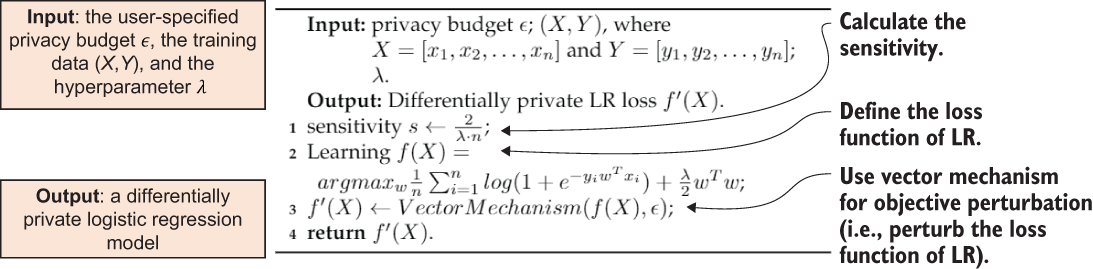
Figure 3.9 How differentially private logistic regression works

Based on the adult dataset we used earlier, let’s continue with our previous scenario by training a logistic regression classification model to predict whether a person makes over $50,000 a year. First, let’s load the training and testing data from the adult dataset.

Listing 3.3 Loading testing and training data

import numpy as np
 
X_train = np.loadtxt("https://archive.ics.uci.edu/ml/machine-learning-
➥ databases/adult/adult.data", 
➥ usecols=(0, 4, 10, 11, 12), delimiter=", ")
 
y_train = np.loadtxt("https://archive.ics.uci.edu/ml/machine-learning-
➥ databases/adult/adult.data", 
➥ usecols=14, dtype=str, delimiter=", ")
 
X_test = np.loadtxt("https://archive.ics.uci.edu/ml/machine-learning-
➥ databases/adult/adult.test", 
➥ usecols=(0, 4, 10, 11, 12), delimiter=", ", skiprows=1)
 
y_test = np.loadtxt("https://archive.ics.uci.edu/ml/machine-learning-
➥ databases/adult/adult.test", 
➥ usecols=14, dtype=str, delimiter=", ", skiprows=1)
 
y_test = np.array([a[:-1] for a in y_test])

For diffprivlib, LogisticRegression works best when the features are scaled to control the norm of the data. To streamline this process, we’ll create a Pipeline in sklearn:

from sklearn.linear_model import LogisticRegression
from sklearn.pipeline import Pipeline
from sklearn.preprocessing import MinMaxScaler
 
lr = Pipeline([
    ('scaler', MinMaxScaler()),
    ('clf', LogisticRegression(solver="lbfgs"))
])

Now let’s first train a regular (non-private) logistic regression classifier and test its accuracy:

lr.fit(X_train, y_train)
 
from sklearn.metrics import accuracy_score
 
print("Non-private test accuracy: %.2f%%" % (accuracy_score(y_test,
➥ lr.predict(X_test)) * 100))

You will have output like the following:

> Non-private test accuracy: 81.04%

To apply differentially private logistic regression, we’ll start by installing the IBM Differential Privacy Library:

!pip install diffprivlib

Using the diffprivlib.models.LogisticRegression module of diffprivlib, we can train a logistic regression classifier while satisfying DP.

If we don’t specify any parameters, the model defaults to epsilon = 1 and data_norm = None. If the norm of the data is not specified at initialization (as in this case), the norm will be calculated on the data when .fit() is first called, and a warning will be thrown because it causes a privacy leak. To ensure no additional privacy leakage, we should specify the data norm explicitly as an argument and choose the bounds independent of the data. For instance, we can use domain knowledge to do that.

Listing 3.4 Training a logistic regression classifier

import diffprivlib.models as dp
dp_lr = Pipeline([
    ('scaler', MinMaxScaler()),
    ('clf', dp.LogisticRegression())
])
 
dp_lr.fit(X_train, y_train)
 
print("Differentially private test accuracy (epsilon=%.2f): %.2f%%" %
➥ (dp_lr['clf'].epsilon, accuracy_score(y_test, 
➥ dp_lr.predict(X_test)) * 100))

The output will look something like the following:

> Differentially private test accuracy (epsilon=1.00): 80.93%

As you can see from the preceding output accuracies, the regular (non-private) logistic regression classifier produces an accuracy of 81.04%; by setting epsilon=1.00, the differentially private logistic regression could achieve an accuracy of 80.93%. Using a smaller epsilon usually leads to better privacy protection but lesser accuracy. For instance, suppose we set epsilon=0.01:

import diffprivlib.models as dp
dp_lr = Pipeline([
    ('scaler', MinMaxScaler()),
    ('clf', dp.LogisticRegression(epsilon=0.01))
])
 
dp_lr.fit(X_train, y_train)
 
print("Differentially private test accuracy (epsilon=%.2f): %.2f%%" %
➥ (dp_lr['clf'].epsilon, accuracy_score(y_test, 
➥ dp_lr.predict(X_test)) * 100))

As expected, the result will look something like this:

> Differentially private test accuracy (epsilon=0.01): 74.01%

3.2.3 Differentially private linear regression

Unlike logistic regression, a linear regression model defines a linear relationship between an observed target variable and multiple explanatory variables in a dataset. It is often used in regression analysis for trend prediction. The most common way to compute such a model is to minimize the residual sum of squares between the observed targets (of explanatory variables) in the dataset and the targets (of explanatory variables) predicted by linear approximation.

Let’s dig into the theoretical foundations. We can formulate the standard problem of liner regression as finding β = arg min_β‖Xβ − y‖², where X is the matrix of explanatory variables, y is the vector of the explained variable, and β is the vector of the unknown coefficients to be estimated.

Ridge regression, a regularized version of linear regression, can be formulated as β^R= arg min_β‖Xβ − y‖² + w²‖β‖², which has a closed form solution: β^R = (X^TX + w²I_p×p)X^Ty, where w is set to minimize the risk of β^R.

The problem of designing a differentially private linear regression becomes designing a differentially private approximation of the second moment matrix. To achieve this, Sheffet [6] proposed an algorithm that adds noise to the second moment matrix using the Wishart mechanism. For more details, you can refer to the original paper, but this is enough for us to proceed.

Let’s consider the scenario of training a linear regression on a diabetes dataset. This is another popular dataset among ML researchers, and you can find more information about it here: https://archive.ics.uci.edu/ml/datasets/diabetes. We will work with the example proposed by scikit-learn (https://scikit-learn.org/stable/auto_examples/linear_model/plot_ols.html), and we’ll use the diabetes dataset to train and test a linear regressor.

We’ll begin by loading the dataset and splitting it into training and testing samples (an 80/20 split):

from sklearn.model_selection import train_test_split
from sklearn import datasets
 
dataset = datasets.load_diabetes()
X_train, X_test, y_train, y_test = train_test_split(dataset.data,
➥ dataset.target, test_size=0.2)
print("Train examples: %d, Test examples: %d" % (X_train.shape[0],
➥ X_test.shape[0]))

You will get a result something like the following, showing the number of samples in the train and test sets:

> Train examples: 353, Test examples: 89

We’ll now use scikit-learn’s native LinearRegression function to establish a non-private baseline for our experiments. We’ll use the r-squared score to evaluate the goodness-of-fit of the model. The r-squared score is a statistical measure that represents the proportion of the variance of a dependent variable that’s explained by an independent variable or variables in a regression model. A higher r-squared score indicates a better linear regression model.

from sklearn.linear_model import LinearRegression as sk_LinearRegression
from sklearn.metrics import r2_score
 
regr = sk_LinearRegression()
regr.fit(X_train, y_train)
baseline = r2_score(y_test, regr.predict(X_test))
print("Non-private baseline: %.2f" % baseline)

The result will look like the following:

> Non-private baseline: 0.54

To apply differentially private linear regression, let’s start by installing the IBM Differential Privacy Library, if you have not done so already:

!pip install diffprivlib

Now let’s train a differentially private linear regressor (epsilon=1.00), where the trained model is differentially private with respect to the training data:

from diffprivlib.models import LinearRegression
 
regr = LinearRegression()
regr.fit(X_train, y_train)
 
print("R2 score for epsilon=%.2f: %.2f" % (regr.epsilon, 
➥ r2_score(y_test, regr.predict(X_test))))
 

You will get an R2 score similar to the following:

> R2 score for epsilon=1.00: 0.48

3.3 Differentially private unsupervised learning algorithms

Unsupervised learning is a type of algorithm that learns patterns from unlabeled data. The feature vectors do not come with class labels or response variables in this type of learning. The target, in this case, is to find the structure of the data.

Clustering is probably the most common unsupervised learning technique, and it aims to group a set of samples into different clusters. Samples in the same cluster are supposed to be relatively similar and different from samples in other clusters (the similarity measure could be the Euclidean distance). k-means clustering is one of the most popular clustering methods, and it’s used in many applications. This section will introduce the differentially private design of k-means clustering, and we’ll walk you through the design process.

3.3.1 Differentially private k-means clustering

We will now moving on to differentially private unsupervised learning algorithms. We’ll start by checking out k-means clustering and how it works.

What is k-means clustering?

At a high level, k-means clustering tries to group similar items in clusters or groups. Suppose we have a set of data points that we want to assign to groups (or clusters) based on their similarity; the number of groups is represented by k.

There are multiple different implementations of k-means, including Lloyd’s, MacQueen’s, and Hartigan-Wong’s k-means. We’ll look at Lloyd’s k-mean algorithm [7], as it is the most widely known implementation of k-means.

In the process of training a k-means model, the algorithm starts with k randomly selected centroid points that represent the k clusters. Then the algorithm iteratively clusters samples to the nearest centroid point and updates the centroid points by calculating the means of the samples that are clustered to the centroid points.

Let’s look at an example. In the fresh produce section of your supermarket you’ll see different kinds of fruits and vegetables. These items are arranged in groups by their types: all the apples are in one place, the oranges are kept together, and so on. You will quickly find that they form groups or clusters, where each of the items is within a group of their kind, forming the clusters.

Implementing differentially private k-means clustering

Now that we’ve outlined k-means clustering, let’s start walking through differentially private k-means clustering. This design follows an algorithm perturbation strategy called DPLloyd [8] (an extension of Lloyd’s k-means), where the Laplace mechanism (i.e., adding Laplacian noise) is applied to the iterative update step in the Lloyd algorithm. In essence, it adds Laplace noise to the intermediate centroids and cluster sizes and produces differentially private k-means models.

Suppose each sample of the k-means clustering is a d-dimensional point, and assume the k-means algorithm has a predetermined number of running iterations, denoted as t. In each iteration of the k-means algorithm, two values are calculated:

• The total number of samples of each cluster C_i, denoted as n_i (i.e., the count queries)

• The sum of the samples of each cluster C_i (to recalculate the centroids), denoted as s_i (i.e., the sum queries)

Then, in k-means, each sample will involve d ⋅ t sum queries and t count queries. Adding or deleting a new sample will change n_i by 1, and this operation could happen in every iteration, so the sensitivity of n_i is t. Suppose the size of each dimension (i.e., feature) of each sample is bounded in the range [−r,r]. Then, by adding or deleting a new sample, the difference of x_i will be d ⋅ r ⋅ t.

As mentioned, we are going to use the algorithm perturbation strategy to design our differentially private k-means clustering algorithm, where the sensitivities of the count queries and the sum queries are calculated. The Laplace mechanism (i.e., adding Laplacian noise) is applied to the iterative update step in the Lloyd algorithm by adding noise to the intermediate centroids and cluster sizes. Figure 3.10 illustrates the pseudocode of the algorithm, which is mostly self-explanatory.

Figure 3.10 How differentially private k-means clustering works

Let’s train a k-means clustering model on the scikit-learn load_digits dataset. We’ll follow the example given by scikit-learn and use the load_digits dataset to train and test a k-means model. As you can see in listing 3.5, we’ll use several different metrics for evaluating the clustering performance. Evaluating the performance of a clustering algorithm is not as trivial as counting the number of errors or the precision and recall of a supervised classification algorithm. As such, we will be looking at homogeneity, completeness, and V-measure scores, as well as adjusted rand index (ARI) and adjusted mutual information (AMI) score. Please refer to the scikit-learn documentation for detailed steps and the mathematical formulation: https://scikit-learn.org/stable/modules/clustering.html#clustering-evaluation.

Listing 3.5 Training a k-means clustering model

import numpy as np
from time import time
from sklearn import metrics
from sklearn.cluster import KMeans
from sklearn.datasets import load_digits
from sklearn.preprocessing import scale
 
X_digits, y_digits = load_digits(return_X_y=True)
data = scale(X_digits)
 
n_samples, n_features = data.shape
n_digits = len(np.unique(y_digits))
labels = y_digits
 
sample_size = 1000
 
print("n_digits: %d, 	 n_samples %d, 	 n_features %d"
      % (n_digits, n_samples, n_features))
> n_digits: 10,  n_samples 1797,  n_features 64
 
print('init		time	inertia	homo	compl	v-meas	ARI	AMI	silhouette')
> nit time inertia homo compl v-meas ARI AMI silhouette
 
def bench_k_means(estimator, name, data):
    t0 = time()
    estimator.fit(data)
    print('%-9s	%.2fs	%i	%.3f	%.3f	%.3f	%.3f	%.3f	%.3f'
          % (name, (time() - t0), estimator.inertia_,
             metrics.homogeneity_score(labels, estimator.labels_),
             metrics.completeness_score(labels, estimator.labels_),
             metrics.v_measure_score(labels, estimator.labels_),
             metrics.adjusted_rand_score(labels, estimator.labels_),
             metrics.adjusted_mutual_info_score(labels,
             estimator.labels_),
             metrics.silhouette_score(data, estimator.labels_,
                                      metric='euclidean',
                                      sample_size=sample_size)))

We’ll now use scikit-learn’s native KMeans function to establish a non-private baseline for our experiments. We will use the k-means++ and random initializations:

bench_k_means(KMeans(init='k-means++', n_clusters=n_digits, n_init=100),
              name="k-means++", data=data)
 
bench_k_means(KMeans(init='random', n_clusters=n_digits, n_init=100),
              name="random", data=data)

The results may look like figure 3.11. As you can see, the preceding code covers different resulting score metrics such as homogeneity, completeness, and so on. Homogeneity, completeness, and V-measure scores are bounded below by 0.0 and above by 1.0, and the higher the value, the better. Intuitively, clustering with a bad V-measure can be qualitatively analyzed by using homogeneity and completeness scores to better determine what kinds of mistakes are being made by the assignment. For the ARI, AMI, and silhouette coefficient scores, the range is -1 to 1. Again, the higher the number, the better. On a final note, lower values generally indicate two largely independent labels, whereas values close to 1 indicate significant agreement.

Figure 3.11 Comparing results: k-means++ vs. random initializations

Now let’s apply differential privacy for k-means clustering:

!pip install diffprivlib 
from diffprivlib.models import KMeans
 
bench_k_means(KMeans(epsilon=1.0, bounds=None, n_clusters=n_digits,
➥ init='k-means++', n_init=100), name="dp_k-means", data=data)

Once the differentially private k-means clustering is applied, you’ll see results like those in figure 3.12. As you can see, dp_k-means provides much more varied results than k-means++ and random initializations, providing better privacy assurance. When you compare the numbers of the different score metrics, you will see how DP affects the final result.

Figure 3.12 Comparing results once the differentially private k-means clustering is applied

We’ve now investigated the design and use of several differentially private ML algorithms, and we’ve gone through some hands-on experiments. In the next section we’ll use differentially private principal component analysis (PCA) as a case study application, and we’ll walk you through the process of designing a differentially private ML algorithm.

3.4 Case study: Differentially private principal component analysis

In previous sections we discussed the DP mechanisms commonly used in today’s applications and the design and usage of various differentially private ML algorithms. In this section we’ll discuss how to design differentially private principal component analysis (PCA) as a case study, to walk you through the process of designing a differentially private ML algorithm. The content in this section is partially published in our paper [9], which you can refer to for further details. The implementation of this case study can be found in the book’s GitHub repository: https://github.com/nogrady/PPML/blob/main/Ch3/distr_dp_pca-master.zip.

NOTE This section aims to walk you through all the mathematical formulations and empirical evaluations of our case study so that you can understand how to develop a differentially private application from scratch. If you do not need to know all these implementation details right now, you can skip to the next chapter and come back to this section later.

3.4.1 The privacy of PCA over horizontally partitioned data

PCA is a statistical procedure that computes a low-dimension subspace from the underlying data and generates a new set of variables that are linear combinations of the original ones. It is widely used in various data mining and ML applications, such as network intrusion detection, recommendation systems, text and image processing, and so on.

In 2016, Imtiaz et al. presented a first-of-its-kind privacy-preserving distributed PCA protocol [10]. Their main idea was to approximate the global PCA by aggregating the local PCA from each data owner, in which the data owner holds horizontally partitioned data. However, their work suffers from excessive running time and utility degradation, while the local principal components fail to provide a good representation of the data. More specifically, their solution requires all data owners to be online and to transfer the local PCA data one by one. This serialized computation made their protocol dependent on the number of data owners, which seriously degraded efficiency and scalability. Also, the local principal components cannot provide a good representation of the utility of the principal components when the amount of data is far less than its number of features.

In our case study, we will assume that the data is horizontally partitioned, which means all the data shares the same features. The number of data owners will be more than hundreds. We’ll presume an untrustworthy data user would like to learn the principal components of the distributed data. An honest but curious intermediary party, named proxy, works between the data user and data owners.

Data owners simultaneously encrypt their own data share and send it to the proxy. The proxy runs a differentially private aggregation algorithm over the encrypted data and sends the output to the data user. The data user then computes the principal components from the output without learning the content of the underlying data.

In our experiments, we will study the running time, utility, and privacy tradeoff of the proposed protocol and compare it with previous work.

Before moving forward with our protocol design, let’s briefly go over the concepts of PCA and homomorphic encryption.

How principal component analysis works

Let’s quickly walk through the mathematical formulation of PCA. Given a square matrix A, an eigenvector v of A is a nonzero vector that does not change the direction when A is applied to it, such that

Av = λv

where λ is a real number scalar, referred to as the eigenvalue. Suppose A ∈ ℝ^(n×n), then it has at most n eigenvectors, and each eigenvector associates with a distinct eigenvalue.

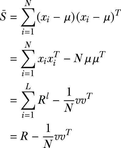
Consider a dataset with N samples x₁, x₂,...,x_N, where each sample has M features (xⁱ ∈ ). A center-adjusted scatter matrix  is computed as follows,

where μ is the mean vector, μ = 1/N ∑^N_(i=1)x_i. By using eigenvalue decomposition (EVD) on , we will have Λ and U, where Λ = diag(λ₁, λ₂,...,λ_M) is a diagonal matrix of eigenvalues.

This can be arranged to a non-increasing order in absolute value; in other words, ‖λ₁‖ ≥ ‖λ₂‖ ≥ ⋯ ≥ ‖λ_M‖, U = [u₁ u₂ ... u_M ] is an M × M matrix where u_j denotes the j^th eigenvector of .

In PCA, each eigenvector represents a principal component.

What is homomorphic encryption?

Homomorphic encryption is an essential building block of this work. In simple terms, it allows computations to be performed over the encrypted data, in which the decryption of the generated result matches the result of operations performed on the plaintext. In this section we will use the Paillier cryptosystem to implement the protocol.

To refresh your memory, the Paillier cryptosystem is a probabilistic asymmetric algorithm for public-key cryptography (a partially homomorphic encryption scheme) introduced by Pascal Paillier.

Let’s consider the function ε_pk[⋅] to be the encryption scheme with public key pk, the function D_sk[⋅] to be the decryption scheme with private key sk. The additive homomorphic encryption can be defined as

where ⊗ denotes the modulo multiplication operator in the encrypted domain and a and b are the plaintext messages. The multiplicative homomorphic encryption is defined as

Since the cryptosystem only accepts integers as input, real numbers should be discretized. In this example, we’ll adopt the following formulation,

where e is the number of bits, and min_F, max_F are the minimal and maximal value of feature F, x is the real number to be discretized, and Discretize_(e,F) (x) takes a value in [0,2^(e-1)].

3.4.2 Designing differentially private PCA over horizontally partitioned data

Let’s first revisit what we want to achieve here (see figure 3.13). Suppose there are L data owners, and each data owner l has a dataset , where M is the number of dimensions and N^l is the number of samples held by l. The horizontal aggregation of X^l, i = 1,2,...,l generates a data matrix X ∈ ℝ^(N×M), where N = ∑^l_(i=1)Nⁱ. Now assume a data user wants to perform PCA on X. To protect the privacy of the original data, data owners would not share the original data with the data user in cleartext form.

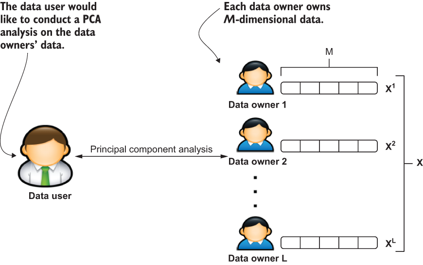
Figure 3.13 The high-level overview of distributed PCA

To accommodate this, we need to design a differentially private distributed PCA protocol that allows data users to perform PCA but to learn nothing except the principal components. Figure 3.14 illustrates one design for a differentially private distributed PCA protocol. In this scenario, data owners are assumed to be honest and not to collude with each other, but the data user is assumed to be untrustworthy and will want to learn more information than the principal components. The proxy works as an honest-but-curious intermediary party who does not collude with the data user or owners.

Figure 3.14 The design of the protocol and how it works

In order to learn the principal components of X, the scatter matrix of X needs to be computed. In the proposed protocol, each data owner l computes a data share of X^l. To prevent the proxy learning the data, each data share is encrypted before it is sent to the proxy. Once the proxy receives the encrypted data share from each data owner, the proxy runs the differentially private aggregation algorithm and sends the aggregated result to the data user. Then the data user constructs the scatter matrix from the result and computes the principal components. Figure 3.14 outlines these steps.

Computing the scatter matrix

Let’s look at the computation of the distributed scatter matrix.

Suppose there are L data owners, and each data owner l has a dataset, , where M is the number of dimensions, and N^l is the number of samples held by l. Each data owner locally computes a data share that contains

where x_i = [x_i1 x_i2... x_iM]^Te. The scatter matrix  can be computed by summing the data share from each data owner:

where

The distributed scatter matrix computation allows each data owner to compute a partial result simultaneously. Unlike other methods [10], this approach reduces the dependence between data owners and allows them to send the data shares simultaneously.

Designing the protocol

It is crucial to prevent any possible data leakage through the proxy, so each individual data share should be encrypted by the data owners. Then the proxy aggregates the received encrypted shares. To prevent the inference from PCA, the proxy adds a noise matrix to the aggregated result, which makes the approximation of the scatter matrix satisfy (ϵ, δ)-DP. The aggregated result is then sent to the data user.

What is (ϵ, δ)-DP? δ is another privacy budget parameter, where, when δ = 0, the algorithm satisfies ϵ-DP, which is a stronger privacy guarantee than (ϵ, δ)-DP with δ > 0. You can find more details about δ in section A.1

This can be seen as the most general relaxation of ϵ-DP, which weakens the definition by allowing an additional small δ density of probability on which the upper bound ε does not hold. If you think of the practicality of DP, this leads to the dilemma of data release. You cannot always be true to the data and protect the privacy of all individuals. There is a tradeoff between the utility of the output and privacy. Especially in the case of outliers, an ϵ private release will have very little utility (as the sensitivity is very large, leading to a lot of noise being added).

Alternatively, you can remove the outliers or clip their values to achieve a more sensible sensitivity. This way the output will have better utility, but it is no longer a true representation of the dataset.

This all leads to (ϵ, δ) privacy. The data user decrypts the result, constructs an approximation of the scatter matrix, and then calculates PCA, as you saw earlier. Let’s walk through the steps:

1. The data user generates a public key pair (pk and sk) for the Paillier cryptosystem and sends pk to the proxy and data owners. In practice, secure distribution of keys is important, but we are not emphasizing it here.

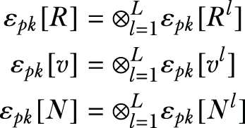
   Thereafter, the data owners compute the share R^l, v^l, l = 1,2,..., L, and send ε_pk[R^l], ε_pk[v^l], ε_pk[N^l] to the proxy.

2. After receiving the encrypted data share from each data owner, the proxy aggregates the shares and applies the symmetric matrix noise to satisfy DP. This process is shown in algorithm 1 in figure 3.15.

Let’s look at algorithm 1 to understand what’s happening here:

1. Lines 2-4: Aggregate the data shares from each data owner.

   

2. Lines 5-7: Construct the noisy ε_pk[v ']. To prevent the data user learning information from v, the proxy generates a noisy ε_pk[v'] by summing a random vector ε_pk[b] with ε_pk[v], such that ε_pk[v'] = ε_pk[v] ⊗ ε_pk[b]. It can be shown that the element v'_ij of v'v'^T is

   

   Both sides of the equation are divided by N, which yields

   

   

   Thus, we have

   

   Recall that, in the Paillier cryptosystem, the multiplicative homomorphic property is defined as

   

   Then, ε_pk[G_ij] is

   

   At this point we can make the exponent be an integer by multiplying b with N. It should be noted that during the encryption, the proxy has to learn N. To achieve this, the proxy sends ε_pk[N] to the data user, and the data user returns N in cleartext once it’s decrypted.

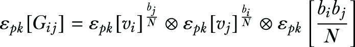
3. Lines 8-10: Apply symmetric matrix to satisfy (ϵ, δ)-DP. The proxy generates G’ ∈ ℝ^M×M, based on the DP parameter (ϵ, δ), and gets ℇ_pk[R’], ℇ_pk[v’], where

   

   

   Then, ℇ_pk[R’], ℇ_pk[v’] are sent to the data user.

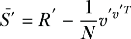
   After receiving the aggregated result from the proxy, ε_pk[N], ε_pk[R’], ε_pk[v’], the data user decrypts each and computes .

   

   With , the data user can proceed to compute the eigenvector and get the principal components.

Figure 3.15 Algorithm 1: DPAggregate

Analyzing the security and privacy

Now let’s determine whether the protocol is secure enough. In our example, the data user is assumed to be untrustworthy, and the proxy is assumed to be honest but curious. Furthermore, we are assuming that the proxy will not collude with the data user or data owners.

To protect the data against the proxy, R^l, v^l, and N^l are encrypted by the data owner. During the protocol execution, the proxy only learns N in plaintext, and it will not disclose the privacy of a single data owner. Without colluding with the data user, the proxy cannot learn the values of R^l, v^l, and N^l. On the other side, the proxy mixes R and v with random noise, to prevent the data user from gaining information other than the principal components.

Of the data received from the proxy, the data user decrypts ε_pk[N], ε_pk[R’], ε_pk[v’] and then proceeds to construct an approximation of the scatter matrix, , in which G’ is the Gaussian symmetric matrix carried by R’. The (ϵ, δ)-DP is closed for the postprocessing algorithm of . Since the proxy is not colluding with the data user, the data user cannot learn the value of R and v. Therefore, the data user learns nothing but the computed principal components.

As a flexible design, this approach can cooperate with different symmetric noise matrices to satisfy (ϵ, δ)-DP. To demonstrate the protocol to you, we implemented the Gaussian mechanism as shown in algorithm 2 (figure 3.16).

Figure 3.16 Algorithm 2: the Gaussian mechanism

It is noteworthy that once the data user learns the private principal components from the protocol, they could release the principal components to the public for further use, which would allow the proxy to access the components. In that case, the proxy would still not have enough information to recover the covariance matrix from a full set of principal components, which implies that the proxy cannot recover the approximation of the covariance matrix with the released private principal components. Moreover, the data user might release a subset (top K ) of principal components rather than the full set of components, which would make it even harder for the proxy to recover the covariance matrix. Without knowing the approximation of the covariance matrix, the proxy could not infer the plain data by removing the added noise.

3.4.3 Experimentally evaluating the performance of the protocol

We’ve discussed the theoretical background of the proposed protocol, so now let’s implement the differentially private distributed PCA (DPDPCA) protocol and evaluate it in terms of efficiency, utility, and privacy. For efficiency, we will measure the run-time efficiency of DPDPCA and compare it to similar work in the literature [10]; this will show that DPDPCA outperforms the previous work.

This experiment will be developed using Python and the Python Paillier homomorphic cryptosystem library published in https://github.com/mikeivanov/paillier.

The dataset and the evaluation methodology

We will use six datasets for the experiments, as shown in table 3.2. The Aloi dataset is a collection of color images of small objects, the Facebook comment volume dataset contains features extracted from Facebook posts, and the Million Song dataset consists of audio features. The cardinalities of Aloi, Facebook, and Million Song are more than 100,000, and the dimensionality of each is less than 100. The CNAE dataset is a text dataset extracted from business documents, and the attributes are the term frequency. The GISETTE dataset contains grayscale images of the highly confusable digits 4 and 9, used in the NIPS 2003 feature selection challenge. ISOLET is a dataset of spoken letters, which records the 26 English letters from 150 subjects, and it has a combination of features like spectral coefficients and contour features. All the datasets, excluding Aloi, are from the UCI ML repository, whereas Aloi is from LIBSVM dataset repository. We’ll evaluate the performance of DPDPCA in terms of SVM classification over the CNAE, GISETTE, and ISOLET datasets.

Table 3.2 A summary of the experimental datasets

For the classification result, we’ll measure the precision, recall, and F1 scores because the datasets are unbalanced. You can refer to the following mathematical formulations for the details of these measurements. In addition, all experiments will be run 10 times, and the mean and standard deviation of the result will be drawn in figures.

The efficiency of the proposed approach

As we’ve mentioned, the previous work suffered from two main problems: the excessive protocol running time and the utility degradation when the local principal components failed to provide good data representation. In this section we’ll compare both protocols in these two aspects. For brevity, we’ll refer to the proposed protocol as “DPDPCA” and the work done by Imtiaz and Sarwate [11] as “PrivateLocalPCA.”

First, we’ll look at the results of the running times of DPDPCA and PrivateLocalPCA. The total running time of DPDPCA included the following:

• The average local computation time of the data owner

• The time of the private aggregation algorithm in the proxy

• The time of performing PCA by the data user

• The data transmission time among parties

For PrivateLocalPCA, the running time started with the first data owner and ended with the last data owner, including the local PCA computation and transmission time. We simulated the data transmission using I/O operations rather than the local network to make the communication consistent and stable. We measured the protocol running time for the different number of data owners, and all samples were distributed evenly to each data owner. The experiment ran on a desktop machine (i7-5820k, 64 GB memory).

The results are shown in figure 3.17. The horizontal axis specifies the number of data owners, and the vertical axis specifies the running time in seconds. You can see that PrivateLocalPCA runs almost linearly upon the number of data owners. That’s because PrivateLocalPCA requires that the local principal components are transmitted through data owners one by one, and the next data owner has to wait for the result from the previous one. Thus, it has a time complexity of O(n), where n is the number of data owners. In contrast, DPDPCA costs far less time than PrivateLocalPCA, given the same number of data owners. The reason is, first, that the distributed scatter matrix computation allows each data owner to compute their local share simultaneously, and second, that the proxy can implement the aggregation of the local shares in parallel, which runs loglinearly upon the number of data owners. Overall, DPDPCA has better scalability than PrivateLocalPCA regarding the number of data owners.

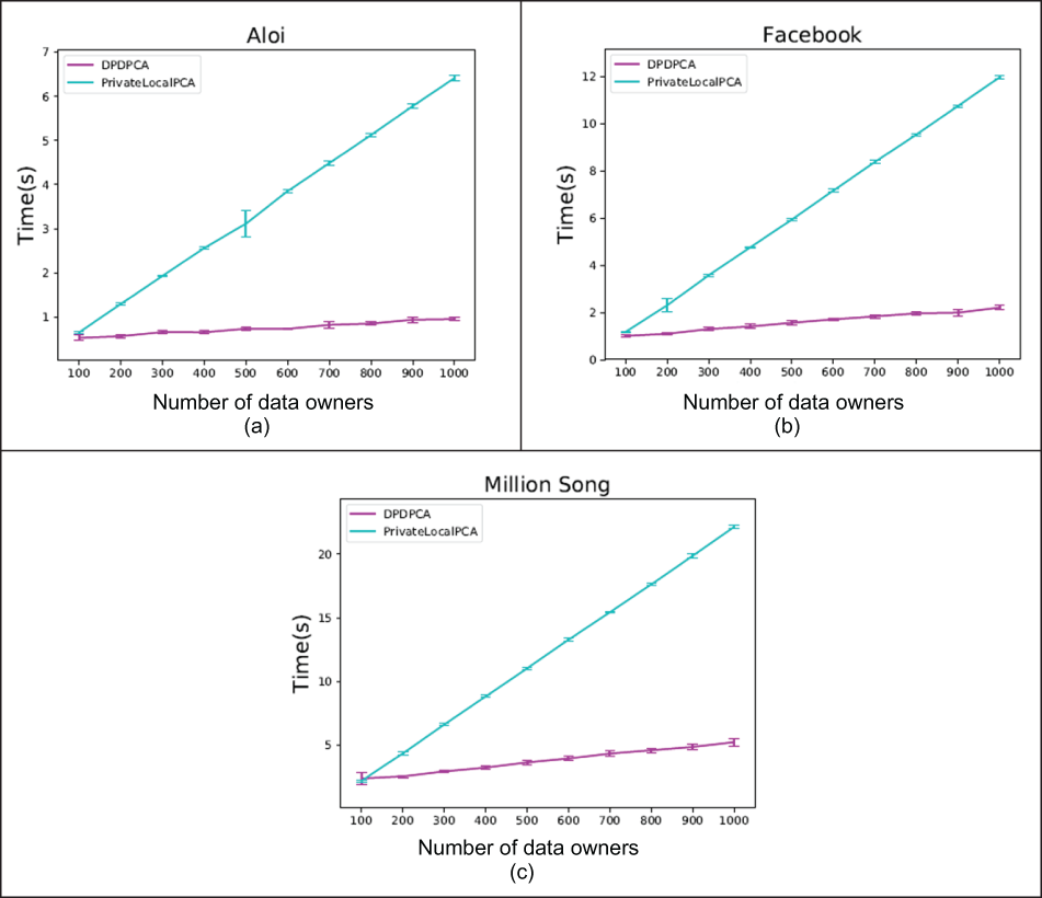
Figure 3.17 Running-time comparison between DPDPCA and PrivateLocalPCA, ∈ = 0.3

The effect on the utility of the application

Next, we’ll explore the utility degradation of PrivateLocalPCA and DPDPCA when the amount of data is far less than the number of features. We are considering a scenario where each data owner holds a dataset where the cardinality may be far smaller than the number of features, such as the images, ratings of music and movies, and personal activity data. To simulate this scenario, we distributed different sized samples to each data owner in the experiment. For PrivateLocalPCA, the variance is not fully preserved because only the first few principal components are used to represent the data.

In contrast, DPDPCA is not affected by the number of samples that each data owner holds, and the local descriptive statistics are aggregated to build the scatter matrix. Thus, the total variance is not lost. In this experiment, we measured the F1 score of the transformed data regarding the different number of private principal components. The number of principal components was determined by each data owner’s rank of the data. Training and testing data were projected to a lower-dimensional space with components from each protocol. Then we used the transformed training data to train an SVM classifier with the RBF kernel and test the classifier with unseen data. To provide ground truth, the noiseless PCA was performed over the training data as well. Also, the same symmetric matrix noise mechanism [10] was applied to DPDPCA to make a fair comparison.

Figure 3.18 shows the results. The horizontal axis specifies the number of samples held by each data owner, and the vertical axis shows the F1 score. You can see that the F1 score of DPDPCA is invariant to the number of samples for the data owner, and the result is compatible with the noiseless PCA, which implies that high utility is maintained. In contrast, the F1 score of PrivateLocalPCA is heavily affected by the number of samples for each data owner, and it cannot maintain the utility with only a few samples. Overall, for the CNAE and GISETTE datasets, the F1 score of DPDPCA outperforms PrivateLocalPCA under all settings.

Figure 3.18 Principal components utility comparison between DPDPCA and PrivateLocalPCA, ∈ = 0.5

The tradeoff between utility and privacy

The other important concern is the tradeoff between utility and privacy. Let’s investigate the tradeoff for DPDPCA by measuring the captured variance of the private principal components using the Gaussian mechanism, where the standard deviation of the additive noise is inversely proportional to ∈. The smaller ∈ is, the more noise is added and the more privacy is gained. The result is shown in figure 3.19, where the horizontal axis specifies ∈, and the vertical axis shows the ratio of the captured variance. In the figure you can see that the variance captured by the Gaussian mechanism almost maintained the same level for the given ∈ range. Moreover, the value of the ratio implies that the Gaussian mechanism captures a large proportion of the variance.

Figure 3.19 Captured variance, δ = 1/N

In conclusion, this case study presents a highly efficient and largely scalable (ϵ, δ)-DP distributed PCA protocol, DPDPCA. As you can see, we considered the scenario where the data is horizontally partitioned and an untrustworthy data user wants to learn the principal components of the distributed data in a short time. We can think of practical applications, such as disaster management and emergency response. Compared to previous work, DPDPCA offers higher efficiency and better utility. Additionally, it can incorporate different symmetric matrix schemes to achieve (ϵ, δ)-DP.

Summary

• DP techniques resist membership inference attacks by adding random noise to the input data, to iterations in the algorithm, or to algorithm output.

• For input perturbation-based DP approaches, noise is added to the data itself, and after the desired non-private computation has been performed on the noisy input, the output will be differentially private.

• For algorithm perturbation-based DP approaches, noise is added to the intermediate values in iterative ML algorithms.

• Output perturbation-based DP approaches involve running the non-private-learning algorithm and adding noise to the generated model.

• Objective perturbation DP approaches entail adding noise to the objective function for learning algorithms, such as empirical risk minimization.

• Differentially private naive Bayes classification is based on Bayes’ theorem and the assumption of independence between every pair of features.

• We can adopt the objective perturbation strategy in designing differentially private logistic regression, where noise is added to the objective function for learning algorithms.

• In differentially private k-means clustering, the Laplace noise is added to the intermediate centroids and cluster sizes and finally produces differentially private k-means models.

• The concept of DP can be used in many distributed ML scenarios, such as PCA, to design highly efficient and largely scalable (ϵ, δ)-DP distributed protocols.