7 Privacy-preserving data mining techniques

This chapter covers

• The importance of privacy preservation in data mining
• Privacy protection mechanisms for processing and publishing data
• Exploring privacy-enhancing techniques for data mining
• Implementing privacy techniques in data mining with Python

So far we have discussed different privacy-enhancing technologies that the research community and the industry have partnered together on. This chapter focuses on how these privacy techniques can be utilized for data mining and management operations. In essence, data mining is the process of discovering new relationships and patterns in data to achieve further meaningful analysis. This usually involves machine learning, statistical operations, and data management systems. In this chapter we will explore how various privacy-enhancing technologies can be bundled with data mining operations to achieve privacy-preserving data mining.

First, we will look at the importance of privacy preservation in data mining and how private information can be disclosed to the outside world. Then we will walk through the different approaches that can be utilized to ensure privacy guarantees in data mining operations, along with some examples. Toward the end of this chapter, we will discuss the recent evolution of data management techniques and how these privacy mechanisms can be instrumented in database systems to design a tailor-made privacy-enriched database management system.

7.1 The importance of privacy preservation in data mining and management

Today’s applications are continually generating large amounts of information, and we all know the importance of privacy protection in this deep learning era. It is similarly important to process, manage, and store the collected information in a time-efficient, secure data processing framework.

Let’s consider a typical deployment of a cloud-based e-commerce application where the users’ private information is stored and processed by the database application (figure 7.1).

Figure 7.1 A typical deployment of an e-commerce web application. All user data, including private information, is stored in a database, and that data will be used by data mining operations.

In e-commerce applications, users connect through web browsers, choose the products or services they want, and make their payments online. All this is recorded on the backend database, including private information such as the customer’s name, address, gender, product preferences, and product types. This information is further processed by data mining and ML operations to provide a better customer experience. For example, the customer’s product preferences can be linked with the choices of other customers to suggest additional products. Similarly, customer addresses can be used to provide location-based services and suggestions. While this approach has numerous benefits for the customers, such as enhanced service quality, it also comes with many privacy concerns.

Let’s take a simple example of a customer who regularly purchases clothes online. In this case, even though the gender may not specifically be mentioned, data mining algorithms might deduce the customer’s gender simply by looking at what type of clothes the customer has purchased in the past. This becomes a privacy concern and is generally termed an inference attack. We will be looking at these attacks in more detail in the next chapter.

Now that most tech giants (such as Google, Amazon, and Microsoft) offer Machine Learning as a Service (MLaaS), small and medium-sized enterprises (SMEs) tend to launch their products based on these services. However, these services are vulnerable to various insider and outsider attacks, as we will discuss toward the end of this chapter. Thus, by linking two or more databases or services together, it is possible to infer more sensitive or private information. For example, an attacker who has access to the zip code and gender of a customer on an e-commerce website can combine that data with the publicly available Group Insurance Commission (GIC) dataset [1], and they might be able to extract the medical records of the individual. Therefore, privacy preservation is of utmost importance in data mining operations.

To that end, in this chapter and the next, we’ll elaborate on the importance of privacy preservation for data mining and management, their applications and techniques, and the challenges in two particular aspects (as depicted in figure 7.2):

• Data processing and mining—Tools and techniques that can be used whenever the collected information is processed and analyzed through various data mining and analytical tools

• Data management—Methods and technologies that can be used to hold, store, and serve collected information for different data processing applications

Figure 7.2 In essence, there are two aspects of privacy preservation when it comes to data mining and management.

Accordingly, we will look at how privacy preservation can be ensured by modifying or perturbing the input data and how we can protect privacy when data is released to other parties.

7.2 Privacy protection in data processing and mining

Data analysis and mining tools are intended to extract meaningful features and patterns from collected datasets, but direct use of data in data mining may result in unwanted data privacy violations. Thus, privacy protection methods utilizing data modification and noise addition techniques (sometimes called data perturbation) have been developed to protect sensitive information from privacy leakage.

However, modifying data may reduce the accuracy of the utility or even make it infeasible to extract essential features. The utility here refers to the data mining task; for example, in the previously mentioned e-commerce application, the mechanism that suggests products to the customer is the utility, and privacy protection methods can be used to protect this data. However, any data transformation should maintain the balance between privacy and the utility of the intended application so that data mining can still be performed on the transformed data.

Let’s briefly look at what data mining is and how privacy regulations come into the picture.

7.2.1 What is data mining and how is it used?

Data mining is the process of extracting knowledge from a collected dataset or set of information. Information systems regularly collect and store valuable information, and the goal of storing information in a datastore is to extract information such as relationships or patterns. To that end, data mining is helpful in discovering new patterns from these datasets. Hence, data mining can be considered the process of learning new patterns or relationships. For instance, in our e-commerce example, a data mining algorithm could be used to determine how likely it is for a customer who purchased baby diapers to also purchase baby wipes. Based on such relationships, service providers can make timely decisions.

Generally, these relationships or patterns can be described with mathematical models that apply to a subset of the original data in the collection. In fact, the identified model can be used in two different ways. First, the model can be used in a descriptive way, where identified relationships between the data in a collection can be turned into human-recognizable descriptions. For example, a company’s current financial situation (whether they are making profits or not) can be described based on the past financial data stored in a dataset. These are called descriptive models, and they usually provide accurate information based on historical data. Predictive models are the second way. Their accuracy may not be very precise, but they can be used to forecast the future based on past data. For example, a question like “If the company invests in this new project, will they will increase their profit margin five years down the line?” can be answered using predictive models.

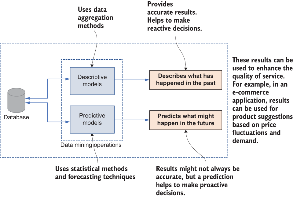
Figure 7.3 Relationships and patterns in data mining can be realized in two different ways.

As shown in figure 7.3, data mining can produce descriptive models and predictive models, and we can apply them for decision making based on the requirements of the underlying application. For example, in e-commerce applications, predictive models can be used to forecast the price fluctuations of a product.

7.2.2 Consequences of privacy regulatory requirements

Traditionally, data security and privacy requirements were set by the data owners (such as organizations on their own) to safeguard the competitive advantage of the products and services they offer. However, data has become the most valuable asset in the digital economy, and many privacy regulations have been imposed by governments to prevent the use of sensitive information beyond its intended purpose. Privacy standards such as HIPAA (Health Insurance Portability and Accountability Act of 1996), PCI-DSS (Payment Card Industry Data Security Standard), FERPA (Family Educational Rights and Privacy Act), and the European Union’s GDPR (General Data Protection Regulation) are commonly adhered to by different organizations.

For instance, regardless of the size of the practice, almost every healthcare provider transmits health information electronically in connection with certain transactions, such as claims, medication records, benefit eligibility inquiries, referral authorization requests, and so on. However, the HIPAA regulations require all these healthcare providers to protect sensitive patient health information from being disclosed without the patient’s consent or knowledge.

In the next section we’ll look at different privacy-preserving data management technologies in detail and discuss their applications and flaws in ensuring these privacy requirements.

7.3 Protecting privacy by modifying the input

Now that you know the basics, let’s get into the details. The well-established privacy-preserving data management (PPDM) technologies can be grouped into several different classes based on how privacy assurance is implemented. We will discuss the first two classes in this chapter; the others will be covered in the next chapter.

The first class of PPDM techniques ensures privacy when data is collected and before it is moved to the datastore. These techniques usually incorporate different randomization techniques at the data collection stage and generate privatized values individually for each record, so original values are never stored. The two most common randomization techniques are modifying data by adding noise with a known statistical distribution and modifying data by multiplying noise with a known statistical distribution.

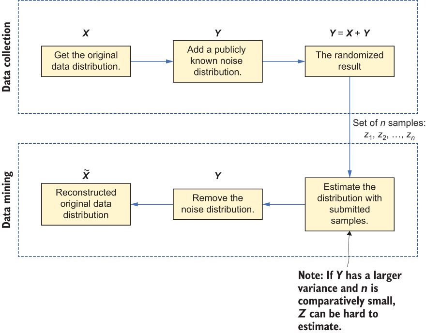
Figure 7.4 Using randomization techniques in data input modification

Figure 7.4 illustrates the first of these two techniques. During the data collection stage, a publicly known noise distribution is added to produce a randomized result. Then, when data mining is involved, we can simply estimate the noise distribution based on the samples, and the original data distribution can be reconstructed. However, it’s important to note that, while the original data distribution may be reconstructed, the original values are not.

7.3.1 Applications and limitations

Now that we have looked at how input can be modified to preserve privacy, let’s look at the merits and demerits of these randomization techniques.

Most importantly, those methods can preserve the statistical properties of the original data distribution even after randomization. This is why they have been used in different privacy-preserving applications, including differential privacy (which we discussed in chapters 2 and 3).

However, since the original data is perturbed and only the data distribution is available (not the individual data), these methods require special data mining algorithms that can extract the necessary information by looking at the distribution. Thus, depending on the application, this method might have a greater effect on the utility.

Tasks like classification and clustering can work well with these input randomization techniques, as they only require access to the data distribution. For example, consider employing such a technique on a medical diagnosis dataset for a disease identification task that is based on specific features or parameters. In such a case, access to the individual records is unnecessary, and the classification can be done based on the data distribution.

7.4 Protecting privacy when publishing data

The next class of PPDM deals with techniques for when data is released to third parties without disclosing the ownership of sensitive information. In this case, data privacy is achieved by applying data anonymization techniques for individual data records before they are released to the outside parties.

As discussed in the previous chapter, removing attributes that can explicitly identify an individual in a dataset is insufficient at this stage. Users in the anonymized data may still be identified by linking them to external data by combining nonsensitive attributes or records. These attributes are called quasi-identifiers.

Let’s consider a scenario we discussed in chapter 6 of combining two publicly available datasets. It is quite straightforward to combine different values in the US Census dataset, such as zip code, gender, and date of birth, with an anonymized dataset from the Group Insurance Commission (GIC). By doing so, someone might be able to extract the medical records of a particular individual. For instance, if Bob knows the zip code, gender, and date of birth of his neighbor Alice, he could combine those two datasets using these three attributes, and he might be able to determine which medical records in the GIC dataset are Alice’s. This is a privacy threat called a linkage or correlation attack, where values in a particular dataset are linked with other sources of information to create more informative and unique entries. PPDM techniques that are used when publishing data usually incorporate one or more data sanitization operations to preserve privacy.

Note If you are not familiar with the GIC dataset, it is an “anonymized” dataset of state employees that shows their every hospital visit in the USA. The goal was to help researchers, and the state spent time removing all key identifiers such as name, address, and social security number.

You may have already noticed that many data sanitization operations are used in practice, but most of these operations can be generalized as one of the following types of operations:

• Generalization—This operation replaces a particular value in a dataset with a more general attribute. For example, the numerical value of a person’s salary, such as $56,000, can be replaced by a range of $50,000-$100,000. In this case, once the value is sanitized, we don’t know the exact value, but we know it is between $50,000 and $100,000.

• This approach can be applied to categorical values as well. Consider the previously mentioned US Census dataset, which has employment details. As shown in figure 7.5, instead of categorizing people into different occupations, we can simply group them as “employed” or “unemployed” without exposing the individual occupations.

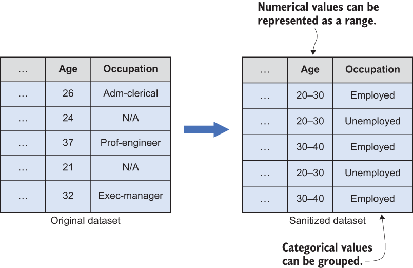
Figure 7.5 Generalization works by grouping the data.

• Suppression—Whereas generalization replaces the original record with a more general representation, the idea of suppression is to remove the record entirely from the dataset. Consider a dataset of hospital medical records. In such a medical database, it is possible to identify an individual based on their name (a sensitive attribute), so we can remove the name attribute from the dataset before publishing it to third parties (see figure 7.6).

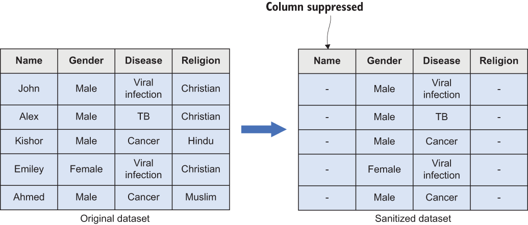
Figure 7.6 Suppression works by removing the original record.

• Perturbation—The other possible data sanitization operation is to replace the individual records with perturbed data that has the same statistical properties, and which can be generated using randomization techniques.

• One possible approach is adding noise to the original values using the techniques we discussed in the previous section, such as additive or multiplicative noise addition. In the example in figure 7.7, the original dataset’s records in the first column are replaced with entirely different values based on random noise.

  

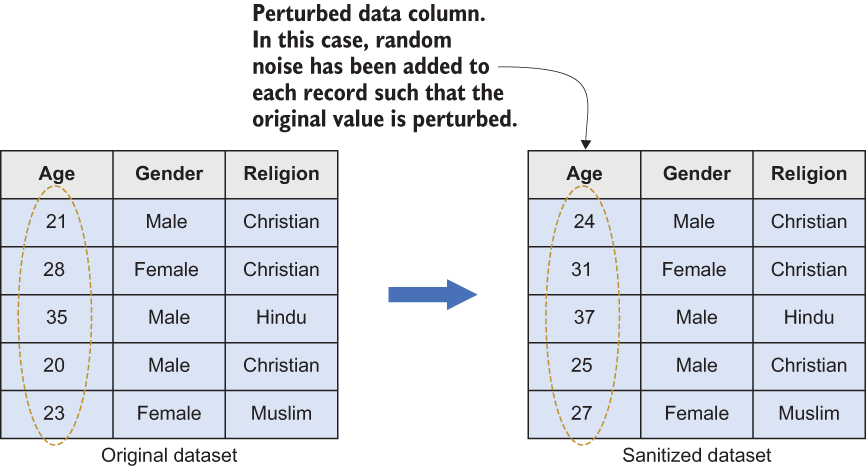
  Figure 7.7 Perturbation works by adding random noise.

  Another approach is to use synthetic data generation techniques as discussed in chapter 6. In that case, a statistical model is built using the original data, and that model can be used to generate synthetic data, which can then replace the original records in the dataset.

  Another possible approach is to use data swapping techniques to accomplish the perturbation. The idea is to swap multiple sensitive attributes in a dataset in order to prevent records from being linked to individuals. Data swapping usually begins by randomly selecting a set of targeted records and then finding a suitable partner for each record with similar characteristics. Once a partner is found, the values are swapped for each other. In practice, data swapping is comparatively time consuming (as it has to loop through many records to find a suitable match), and it requires additional effort to perturb the data.

• Anatomization—Another possible sanitization approach is to separate the sensitive attributes and quasi-identifiers into two separate datasets. In this case, the original values remain the same, but the idea is to make it harder to link them together and identify an individual. Consider the medical dataset we discussed earlier in this list. As shown in figure 7.8, the original dataset can be separated into two distinct datasets: sensitive attributes (e.g., name, religion) and quasi-identifiers (e.g., gender, disease).

  

  Figure 7.8 Using the anatomization approach

7.4.1 Implementing data sanitization operations in Python

In this section we’ll implement these different data sanitization techniques in Python. For this example, we’ll use a real-world dataset [2] that Barry Becker originally extracted from the 1994 US Census database. The dataset contains 15 different attributes, and we’ll first look at how the dataset is arranged. Then we’ll apply different sanitization operations, as depicted in figure 7.9.

Figure 7.9 The order and techniques used in this section’s Python code

First, we need to import the necessary libraries. If you are already familiar with the following packages, you probably have everything installed.

We’ll install these libraries using the pip command:

pip install sklearn-pandas

Once everything is installed, import the following packages to the environment:

import pandas as pd
import numpy as np
import scipy.stats
import matplotlib.pyplot as plt
from sklearn_pandas import DataFrameMapper
from sklearn.preprocessing import LabelEncoder

Now let’s load the dataset and see what it looks like. You can directly download the dataset from the book’s code repository (http://mng.bz/eJYw).

df = pd.read_csv('./Data/all.data.csv')
df.shape
df.head()

With the df.shape() command, you can obtain the dimensionality (number of rows and columns) of the data frame. As you’ll see, this dataset contains 48,842 records categorized in 15 different attributes. You can use the df.head() command to list the first five rows of the dataset, as shown in figure 7.10.

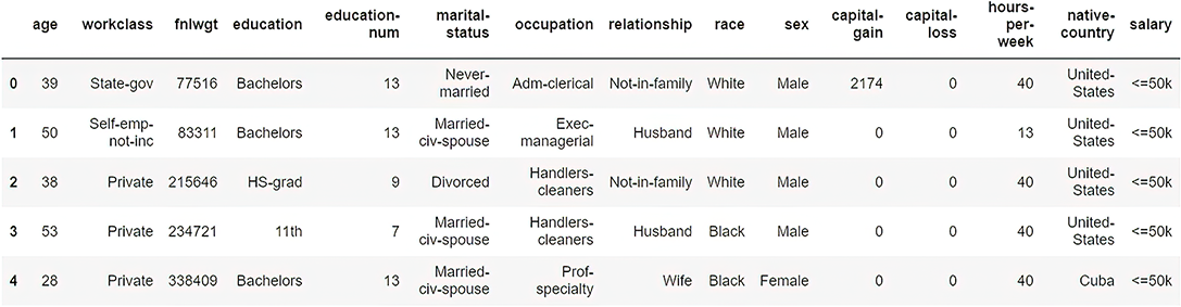
Figure 7.10 First five records of the US Census dataset

You may have noticed that there are some sensitive attributes, such as relationship, race, sex, native-country, and the like, that need to be anonymized. Let’s first apply suppression to some of the attributes so that they can be removed:

df.drop(columns=["fnlwgt", "relationship"], inplace=True)

Try df.head() again and see what has been changed.

Working with categorical values

If you look closely at the race column, you’ll see categorical values such as White, Black, Asian-Pac-Islander, Amer-Indian-Eskimo, and so on. Thus, in terms of privacy preservation, we need to generalize these columns. For that, we will use DataFrameMapper() in sklearn_pandas, which allows us to transform the tuples into encoded values. In this example, we are using LabelEncoder():

encoders = [(["sex"], LabelEncoder()), (["race"], LabelEncoder())]
mapper = DataFrameMapper(encoders, df_out=True)
new_cols = mapper.fit_transform(df.copy())
df = pd.concat([df.drop(columns=["sex", "race"]), new_cols], axis="columns")

Now check the results with df.head() again. It will list the first five rows of the dataset, as shown in figure 7.11.

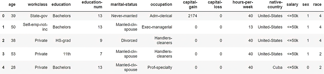
Figure 7.11 Resultant dataset with encoded values

We generalized both the sex and race columns so that no one can have any idea what the gender and race of an individual are.

Working with continuous values

Continuous values such as age can still leak some information about the individuals, as we’ve already discussed. And even though the race is encoded (remember, race is a categorical value), someone could combine a couple of records to obtain more informed results. So let’s apply the perturbation technique to anonymize age and race, as shown in the following listing.

Listing 7.1 Perturbing age and race

categorical = ['race']
continuous = ['age']
unchanged = []

for col in list(df):
    if (col not in categorical) and (col not in continuous):
        unchanged.append(col)

best_distributions = []
for col in continuous:
    data = df[col]
    best_dist_name, best_dist_params = best_fit_distribution(data, 500)
    best_distributions.append((best_fit_name, best_fit_params))

For the continuous variable age, we are using a function called best_fit_ distribution(), which loops through a list of continuous functions to find the best fit function that has the smallest error. Once the best fit distribution is found, we can use it to approximate a new value for the age variable.

For the categorical variable race, we first determine how often a unique value appears in the distribution using value_counts(), and then we use np.random .choice() to generate a random value that has the same probability distribution.

All of this can be wrapped up in a function, as in the following listing.

Listing 7.2 Perturbation for both numerical and categorical values

def perturb_data(df, unchanged_cols, categorical_cols, 
    ➥ continuous_cols, best_distributions, n, seed=0):
    np.random.seed(seed)
    data = {}

    for col in categorical_cols:
        counts = df[col].value_counts()
        data[col] = np.random.choice(list(counts.index),
        ➥ p=(counts/len(df)).values, size=n)

    for col, bd in zip(continuous_cols, best_distributions):
        dist = getattr(scipy.stats, bd[0])        
        data[col] = np.round(dist.rvs(size=n, *bd[1]))
        
        
    for col in unchanged_cols:
        data[col] = df[col]
   
    return pd.DataFrame(data, columns=unchanged_cols+categorical_cols+continuous_cols)    

gendf = perturb_data(df, unchanged, categorical, continuous,
➥ best_distributions, n=48842)

The result of using the gendf.head() command is shown in figure 7.12.

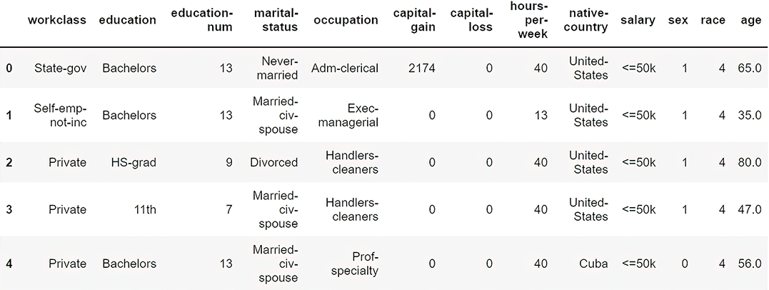
Figure 7.12 Resultant dataset after perturbing both numerical and categorical values

Look closely at the last two columns. The age and race values have been replaced with randomly generated data following the same probability distribution as in the original data. Thus, this dataset can now be treated as privacy preserved.

We have now discussed data sanitization operations that are commonly used in various privacy-preserving applications. Next, we’ll look into how we can apply those operations in practice. We already covered the basics of k-anonymity in section 6.2.2; now, we’ll extend the discussion. The next section covers the k-anonymity privacy model in detail, along with its code implementation in Python.

First, though, let’s recap this section’s sanitization operations in an exercise.

Exercise 1

Consider a scenario where a data mining application is linked with an organization’s employee database. For brevity, we will consider the attributes in table 7.1.

Table 7.1 Employee database of an organization

Now try to answer the following questions to make this dataset privacy-preserved:

• Which attributes can be sanitized using generalization operation? How?

• Which attributes can be sanitized using suppression operation? How?

• Which attributes can be sanitized using perturbation operation? How?

• Does anatomization work in this example? Why?

7.4.2 k-anonymity

One of the most common and widely adopted privacy models that can be used to anonymize a dataset is k-anonymity. Latanya Sweeney and Pierangela Samarati initially proposed it in the late 1990s in their seminal work, “Protecting privacy when disclosing information” [3]. It is a simple yet powerful tool that emphasizes that for a record in a dataset to be indistinguishable, there have to be at least k individual records sharing the same set of attributes that could be used to identify the record (quasi-identifiers) uniquely. In simple terms, a dataset is said to be k-anonymous if it has at least k similar records sharing the same sensitive attributes. We will look into this with an example to better understand how it works.

What is k and how it can be applied?

The value k is typically used to measure privacy, and it is harder to de-anonymize records when the value of k is higher. However, when the k value increases, the utility usually decreases, because the data becomes more generalized.

Many different algorithms have been proposed to achieve k-anonymity, but the vast majority of them apply sanitization operations such as suppression and generalization to achieve the required level of privacy. Figure 7.13 illustrates how to define sensitive and non-sensitive attributes in a dataset, which can be sanitized with k-anonymity in practice.

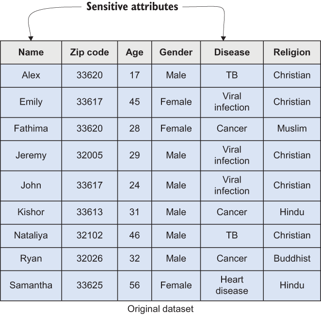
Figure 7.13 Sample dataset defining the sensitive and non-sensitive attributes

There are a couple of important and sensitive attributes and quasi-identifiers in this case. Thus, when we apply k-anonymity, it is vital to make sure that all the records are anonymized enough to make it hard for data users to de-anonymize the records.

Note The sensitivity of an attribute typically depends on the application’s requirements. Attributes that are very sensitive in some cases might be non-sensitive in other application domains.

Let’s consider the dataset shown in figure 7.14. As you can see, the name and religion attributes are sanitized with suppression, while zip code and age are generalized. If you look into that closer, you may realize that it is 2-anonymized (k = 2), meaning there are at least two records in each group. Let’s take the first two records in the table as an example. As you can see, those records are in the same group, making the zip code, age, and gender the same for both; the only difference is the disease.

Figure 7.14 Using generalization and suppression

Now let’s consider a scenario where Bob knows his friend resides in the 32314 zip code, and he is 34 years old. Just by looking at the dataset, Bob cannot distinguish whether his friend has a viral infection or cancer. That is how k-anonymity works. The original information is sanitized and hard to reproduce, but the results can still be used in data mining operations. In the previous example, k = 2, but when we increase the k, it’s even harder to reproduce the original records.

K-anonymity does not always work

While k-anonymity is a powerful technique, it has some direct and indirect drawbacks. Let’s try to understand these flaws to see how k-anonymity is vulnerable to different types of attacks:

• Importance of wisely selecting sensitive attributes—In k-anonymity, the selection of sensitive attributes has to be performed carefully. Still, those selected attributes must not reveal the information of already anonymized attributes. For example, certain diseases can be widespread in certain areas and age groups, so someone might be able to identify the disease by referring to the area or age group. To avoid such scenarios, it is essential to tune the level of suppression and generalization on those attributes of interest. For example, instead of changing the zip code to 32***, you might be able to suppress it to 3****, making the original value harder to guess.

• Importance of having profoundly diversified data in the group—The diversity of the data has major consequences for k-anonymity. Broadly speaking, there are two significant concerns in k-anonymity in terms of having well-represented diversified data. The first is that each represented individual has one and only one record in the group or equivalence classes. The second arises when the values of the sensitive attributes are the same for all the other k-1 records in the group or equivalence class, which could lead to identifying any individual in the group. Regardless of whether the sensitive attributes are the same, these concerns can make k-anonymity vulnerable to different types of attacks.

• Importance of managing data at a low dimension—When the data dimension is high, it is hard for k-anonymity to maintain the required level of privacy within practical limits. For example, stringing multiple data records together can sometimes uniquely identify an individual for data types such as location data. On the other hand, when the data records are sparsely distributed, a lot of noise must be added to group them in order to achieve k-anonymity.

Now let’s look at the attacks we mentioned and how these attacks work. As shown in figure 7.15, there are a set of prerequisites for these attacks to work. For instance, for some attacks, such as the homogeneity attack, to work, the value of the sensitive attributes has to be the same for other records within the group of a k-anonymized dataset.

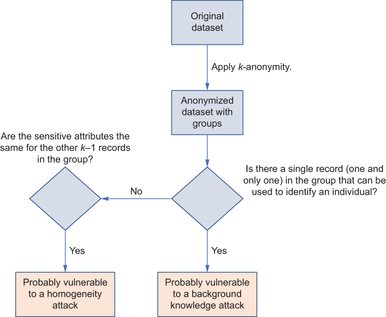
Figure 7.15 A flow diagram explaining possible flaws in k-anonymity leading to different attacks

Let’s look at the example depicted in figure 7.16. Suppose Alice knows her neighbor Bob has been admitted to the hospital, and they both live in the 33718 zip code. In addition, Bob is 36 years old. With that available information, Alice can infer that Bob probably has cancer. This is called a homogeneity attack, where the attacker uses already available information to find a group of records that an individual belongs to.

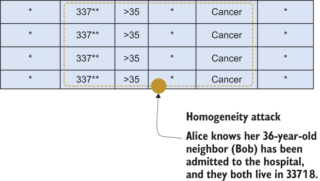
Figure 7.16 Homogeneity attack

Alternatively, this could lead to a background knowledge attack, where an attacker uses external background information to identify an individual in a dataset (see figure 7.17). Suppose Alice has a Japanese friend, Sara, who is 26 years old and currently resides in the 33613 zip code. She also knows that Japanese people have a very low heart disease mortality rate. Given this, she could conclude that her friend is probably suffering from a viral infection.

Figure 7.17 Background knowledge attack

As you can see, we can prevent attacks resulting from attribute disclosure problems by increasing the diversity of the sensitive values within the equivalence group.

7.4.3 Implementing k-anonymity in Python

Now let’s implement k-anonymity in code. For this, we’ll use the cn-protect [4] package in Python. (At the time of publishing, the CN-Protect library has been acquired by Snowflake, and the library is no longer publicly accessible.) You can install it using the following pip code:

pip install cn-protect

Once it is ready, you can load our cleaned-up version of the US Census dataset along with the following listed packages. This version of the dataset is available in the code repository for you to download (http://mng.bz/eJYw).

Listing 7.3 Importing the dataset and applying k-anonymity

import pandas as pd
import matplotlib.pyplot as plt
import seaborn as sns
from cn.protect import Protect
sns.set(style="darkgrid")

df = pd.read_csv('./Data/all.data.csv')

df.shape
df.head()

The results will look like figure 7.18.

Figure 7.18 The first few records of the imported dataset

Using the Protect class, we can first define what the quasi-identifiers are:

prot = Protect(df)
prot.itypes.age = 'quasi'
prot.itypes.sex = 'quasi'

You can look at the types of the attributes using the prot .itypes command, as shown in figure 7.19.

Figure 7.19 Dataset attributes defining quasi-identifiers

Now it’s time to set the privacy parameters. In this example, we are using k-anonymity, so let’s set the k value to be 5:

prot.privacy_model.k = 5

Once it is set, you can see the results by using the prot.privacy_ model command. The result should be something like the following:

<KAnonymity: {'k': 5}>

You can observe the resultant dataset with the following code snippet (see figure 7.20):

prot_df = prot.protect()
prot_df

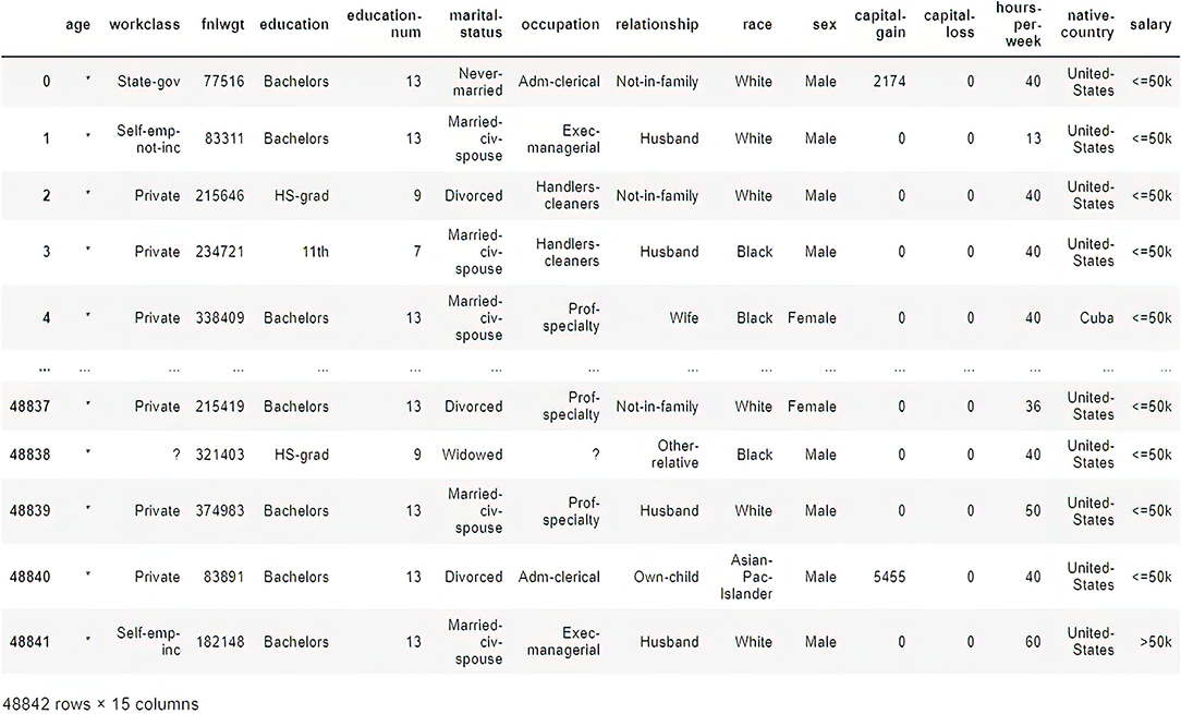
Figure 7.20 A 5-anonymized US Census dataset

Closely look at the resultant age and sex attributes. The dataset is now 5-anonymized. Try it yourself by changing the parameters.

Exercise 2

Consider a scenario where a data mining application involves the following loan information database from a mortgage company. Assume the dataset shown in table 7.2 has many attributes (including mortgage history, loan risk factors, and so on) and records, even though the table only shows a few of them. In addition, the dataset is already 2-anonymized (k = 2).

Table 7.2 Simplified employee database

Now try to answer the following questions to see whether this anonymized dataset still leaks some important information:

• Suppose John knows his neighbor Alice applied for a mortgage and they both live in the 33617 zip code? What information can John deduce?

• If Alice is an African American woman, what additional information can John learn?

• How can you protect this dataset such that John cannot learn anything beyond Alice’s zip code and race?

Summary

• Adopting privacy preservation techniques in data mining and management operations is not a choice. More than ever, it’s a necessity for today’s data-driven applications.

• Privacy preservation in data mining can be achieved by modifying the input data with different noise addition techniques.

• Different data sanitization operations (generalization, suppression, perturbation, anatomization) can be used when publishing data to protect privacy in data mining applications.

• Data sanitization operations can be implemented in different ways depending on the application’s requirements.

• K-anonymity is a widely used privacy model that can be implemented in data mining operations. It allows us to apply various sanitization operations while providing flexibility.

• Although k-anonymity is a powerful technique, it has some direct and indirect drawbacks.

• In a homogeneity attack, the attacker uses already available information to find a group of records that an individual belongs to.

• In a background knowledge attack, the attacker uses external background information to identify an individual in a dataset.