
Chapter 2. Expressing Meaning
In the previous chapter we showed you a simple yet flexible data structure for describing restaurants, bars, and music venues. In this chapter we will develop some code to efficiently handle these types of data structures. But before we start working on the code, let’s see if we can make our data structure a bit more robust.
In its current form, our “fully parameterized venue” table allows us to represent arbitrary facts about food and music venues. But why limit the table to describing just these kinds of items? There is nothing specific about the form of the table that restricts it to food and music venues, and we should be able to represent facts about other entities in this same three-column format.
In fact, this three-column format is known as a triple, and it forms the fundamental building block of semantic representations. Each triple is composed of a subject, a predicate, and an object. You can think of triples as representing simple linguistic statements, with each element corresponding to a piece of grammar that would be used to diagram a short sentence (see Figure 2-1).
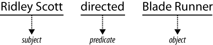
Generally, the subject in a triple corresponds to an entity—a “thing” for which we have a conceptual class. People, places, and other concrete objects are entities, as are less concrete things like periods of time and ideas. Predicates are a property of the entity to which they are attached. A person’s name or birth date or a business’s stock symbol or mailing address are all examples of predicates. Objects fall into two classes: entities that can be the subject in other triples, and literal values such as strings or numbers.
Multiple triples can be tied together by using the same subjects and objects in different triples, and as we assemble these chains of relationships, they form a directed graph. Directed graphs are well-known data structures in computer science and mathematics, and we’ll be using them to represent our data.
Let’s apply our graph model to our venue data by relaxing the meaning of the first column and asserting that IDs can represent any entity. We can then add neighborhood information to the same table as our restaurant data (see Table 2-1).
| Subject | Predicate | Object |
| S1 | Cuisine | “Deli” |
| S1 | Price | “$” |
| S1 | Name | “Deli Llama” |
| S1 | Address | “Peachtree Rd” |
| S2 | Cuisine | “Chinese” |
| S2 | Price | “$$$” |
| S2 | Specialty Cocktail | “Scorpion Bowl” |
| S2 | DJ? | “No” |
| S2 | Name | “Peking Inn” |
| S2 | Address | “Lake St” |
| S3 | Live Music? | “Yes” |
| S3 | Music Genre | “Jazz” |
| S3 | Name | “Thai Tanic” |
| S3 | Address | “Branch Dr” |
| S4 | Name | “North Beach” |
| S4 | Contained-by | “San Francisco” |
| S5 | Name | “SOMA” |
| S5 | Contained-by | “San Francisco” |
| S6 | Name | “Gourmet Ghetto” |
| S6 | Contained-by | “Berkeley” |
Now we have venues and neighborhoods represented using the same model, but nothing connects them. Since objects in one triple can be subjects in another triple, we can add assertions that specify which neighborhood each venue is in (see Table 2-2).
| Subject | Predicate | Object |
| S1 | Has Location | S4 |
| S2 | Has Location | S6 |
| S3 | Has Location | S5 |
Figure 2-2 is a diagram of some of our triples structured as a graph, with subjects and objects as nodes and predicates as directed arcs.

Now, by following the chain of assertions, we can determine that it is possible to eat cheaply in San Francisco. You just need to know where to look.
An Example: Movie Data
We can use this triple model to build a simple representation of a
movie. Let’s start by representing the title of the movie
Blade Runner with the triple
(blade_runner name "Blade
Runner"). You can think of this triple as an arc representing
the predicate called name, connecting the subject
blade_runner to an object, in this case a string,
representing the value “Blade Runner” (see Figure 2-3).

Now let’s add the release date of the film. This can be done with
another triple (blade_runner
release_date "June 25, 1982"). We
use the same ID blade_runner, which indicates that
we’re referring to the same subject when making these statements. It is by
using the same IDs in subjects and objects that a graph is
built—otherwise, we would have a bunch of disconnected facts and no way of
knowing that they concern the same entities.
Next, we want to assert that Ridley Scott directed the movie. The
simplest way to do this would be to add the triple
(blade_runner directed_by
"Ridley Scott"). There is a problem with this approach,
though—we haven’t assigned Ridley Scott an ID, so he can’t be the source
of new assertions, and we can’t connect him to other movies he has
directed. Additionally, if there happen to be other people named “Ridley
Scott”, we won’t be able to distinguish them by name alone.
Ridley Scott is a person and a director, among other things, and
that definitely qualifies as an entity. If we give him the ID
ridley_scott, we can assert some facts about him:
(ridley_scott name "Ridley
Scott"), and (blade_runner
directed_by ridley_scott). Notice that we reused the
name property from earlier. Both entities, “Blade
Runner” and “Ridley Scott”, have names, so it makes sense to reuse the
name property as long as it is consistent with other
uses. Notice also that we asserted a triple that connected two entities,
instead of just recording a literal value. See Figure 2-4.

Building a Simple Triplestore
In this section we will build a simple, cross-indexed triplestore. Since there are many excellent semantic toolkits available (which we will explore in more detail in later chapters), there is really no need to write a triplestore yourself. But by working through the scaled-down code in this section, you will gain a better understanding of how these systems work.
Our system will use a common triplestore design: cross-indexing the subject, predicate, and object in three different permutations so that all triple queries can be answered through lookups. All the code in this section is available to download at http://semprog.com/psw/chapter2/simpletriple.py. You can either download the code and just read the section to understand what it’s doing, or you can work through the tutorial to create the same file.
The examples in this section and throughout the book are in Python. We chose to use Python because it’s a very simple language to read and understand, it’s concise enough to fit easily into short code blocks, and it has a number of useful toolkits for semantic web programming. The code itself is fairly simple, so programmers of other languages should be able to translate the examples into the language of their choice.
Indexes
To begin with, create a file called simplegraph.py. The first thing we’ll do is create a class that will be our triplestore and add an initialization method that creates the three indexes:
class SimpleGraph:
    def __init__(self):
        self._spo = {}
        self._pos = {}
        self._osp = {}
Each of the three indexes holds a different permutation of each
triple that is stored in the graph. The name of the index indicates the
ordering of the terms in the index (i.e., the pos
index stores the predicate, then the
object, and then the subject, in that order). The index is structured
using a dictionary containing dictionaries that in turn contain sets,
with the first dictionary keyed off of the first term, the second
dictionary keyed off of the second term, and the set containing the
third terms for the index. For example, the pos index
could be instantiated with a new triple like so:
self._pos = {predicate:{object:set([subject])}}A query for all triples with a specific predicate and object could be answered like so:
for subject in self._pos[predicate][object]: yield (subject, predicate, object)
Each triple is represented in each index using a different permutation, and this allows any query across the triples to be answered simply by iterating over a single index.
The add and remove Methods
The add method permutes the subject, predicate,
and object to match the ordering of each index:
    def add(self, (sub, pred, obj)):
        self._addToIndex(self._spo, sub, pred, obj)
        self._addToIndex(self._pos, pred, obj, sub)
        self._addToIndex(self._osp, obj, sub, pred)
The _addToIndex method adds the terms to the index, creating a dictionary and set
if the terms are not already in the index:
    def _addToIndex(self, index, a, b, c):
        if a not in index: index[a] = {b:set([c])}
        else:
            if b not in index[a]: index[a][b] = set([c])
            else: index[a][b].add(c)
The remove method finds all triples that match a pattern, permutes them, and
removes them from each index:
    def remove(self, (sub, pred, obj)):
        triples = list(self.triples((sub, pred, obj)))
        for (delSub, delPred, delObj) in triples:
            self._removeFromIndex(self._spo, delSub, delPred, delObj)
            self._removeFromIndex(self._pos, delPred, delObj, delSub)
            self._removeFromIndex(self._osp, delObj, delSub, delPred)
The _removeFromIndex walks down the index, cleaning up empty intermediate
dictionaries and sets while removing the terms of the triple:
    def _removeFromIndex(self, index, a, b, c):
        try:
            bs = index[a]
            cset = bs[b]
            cset.remove(c)
            if len(cset) == 0: del bs[b]
            if len(bs) == 0: del index[a]
        # KeyErrors occur if a term was missing, which means that it wasn't a
        # valid delete:
        except KeyError:
            pass
Finally, we’ll add methods for loading and saving the triples in the graph to
comma-separated files. Make sure to import the csv
module at the top of your file:
    def load(self, filename):
        f = open(filename, "rb")
        reader = csv.reader(f)
        for sub, pred, obj in reader:
            sub = unicode(sub, "UTF-8")
            pred = unicode(pred, "UTF-8")
            obj = unicode(obj, "UTF-8")
            self.add((sub, pred, obj))
        f.close()

     def save(self, filename):
        f = open(filename, "wb")
        writer = csv.writer(f)
        for sub, pred, obj in self.triples((None, None, None)):
            writer.writerow([sub.encode("UTF-8"), pred.encode("UTF-8"),
                obj.encode("UTF-8")])
        f.close()
Querying
The basic query method takes a (subject, predicate, object)
pattern and returns all triples that match the pattern. Terms in the triple that are set to
None are treated as wildcards. The
triples method determines which index to use based on
which terms of the triple are wildcarded, and then iterates over the
appropriate index, yielding triples that match the pattern:
    def triples(self, (sub, pred, obj)):
        # check which terms are present in order to use the correct index:
        try:
            if sub != None:
                if pred != None:
                    # sub pred obj
                    if obj != None:
                        if obj in self._spo[sub][pred]:
                            yield (sub, pred, obj)
                    # sub pred None
                    else:
                        for retObj in self._spo[sub][pred]:
                             yield (sub, pred, retObj)
                else:
                    # sub None obj
                    if obj != None:
                        for retPred in self._osp[obj][sub]:
                             yield (sub, retPred, obj)
                    # sub None None
                    else:
                        for retPred, objSet in self._spo[sub].items():
                            for retObj in objSet:
                                yield (sub, retPred, retObj)
            else:
                if pred != None:
                    # None pred obj
                    if obj != None:
                        for retSub in self._pos[pred][obj]:
                            yield (retSub, pred, obj)
                    # None pred None
                    else:
                        for retObj, subSet in self._pos[pred].items():
                            for retSub in subSet:
                                yield (retSub, pred, retObj)
                else:
                    # None None obj
                    if obj != None:
                        for retSub, predSet in self._osp[obj].items():
                            for retPred in predSet:
                                yield (retSub, retPred, obj)
                    # None None None
                    else:
                        for retSub, predSet in self._spo.items():
                            for retPred, objSet in predSet.items():
                                for retObj in objSet:
                                    yield (retSub, retPred, retObj)
        # KeyErrors occur if a query term wasn't in the index,
        # so we yield nothing:
        except KeyError:
            pass
Now, we’ll add a convenience method for querying a single value of a single triple:
    def value(self, sub=None, pred=None, obj=None):
         for retSub, retPred, retObj in self.triples((sub, pred, obj)):
             if sub is None: return retSub
             if pred is None: return retPred
             if obj is None: return retObj
             break
         return None
That’s all you need for a basic in-memory triplestore. Although you’ll see more sophisticated implementations throughout this book, this code is sufficient for storing and querying all kinds of semantic information. Because of the indexing, the performance will be perfectly acceptable for tens of thousands of triples.
Launch a Python prompt to try it out:
>>> from simplegraph import SimpleGraph
>>> movie_graph=SimpleGraph()
>>> movie_graph.add(('blade_runner','name','Blade Runner'))
>>> movie_graph.add(('blade_runner','directed_by','ridley_scott'))
>>> movie_graph.add(('ridley_scott','name','Ridley Scott'))
>>> list(movie_graph.triples(('blade_runner','directed_by',None)))
[('blade_runner', 'directed_by', 'ridley_scott')]
>>> list(movie_graph.triples((None,'name',None)))
[('ridley_scott', 'name', 'Ridley Scott'), ('blade_runner', 'name', 'Blade Runner')]
>>> movie_graph.value('blade_runner','directed_by',None)
ridley_scott
Merging Graphs
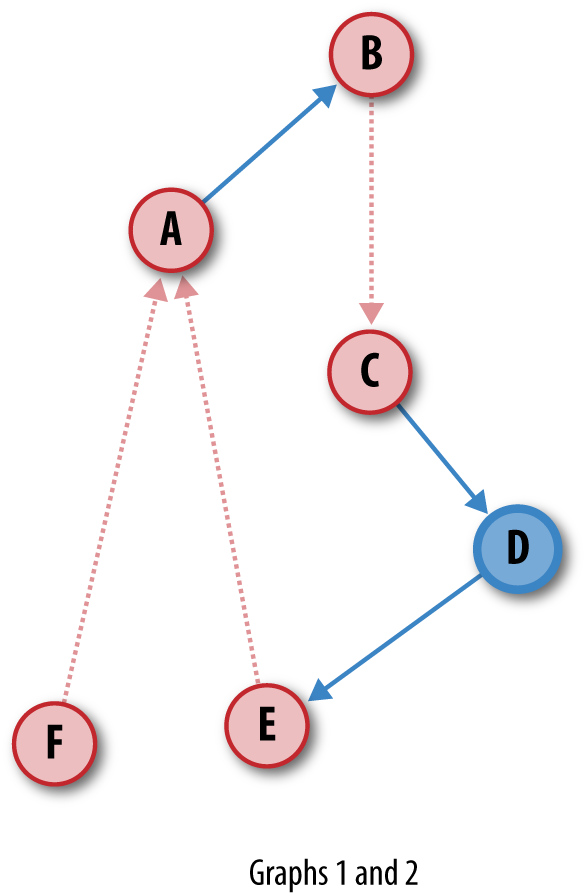
One of the marvelous properties of using graphs to model information is that if you have two separate graphs with a consistent system of identifiers for subjects and objects, you can merge the two graphs with no effort. This is because nodes and relationships in graphs are first-class entities, and each triple can stand on its own as a piece of meaningful data. Additionally, if a triple is in both graphs, the two triples merge together transparently, because they are identical. Figures 2-5 and 2-6 illustrate the ease of merging arbitrary datasets.

In the case of our simple graph, this example will merge two graphs into a single third graph:
>>> graph1 = SimpleGraph()
>>> graph2 = SimpleGraph()
... load data into the graphs ...
>>> mergegraph = SimpleGraph()
>>> for sub, pred, obj in graph1:
...     mergegraph.triples((None, None, None)).add((sub, pred, obj))
>>> for sub, pred, obj in graph2:
...     mergegraph.triples((None, None, None)).add((sub, pred, obj))
Adding and Querying Movie Data
Now we’re going to load a large set of movies, actors, and
directors. The movies.csv file available at http://semprog.com/psw/chapter2/movies.csv
contains over 20,000 movies and is taken from Freebase.com. The predicates that
we’ll be using are name, directed_by for directors, and
starring for actors. The IDs for all of the entities
are the internal IDs used at Freebase.com. Here’s how we load it
into a graph:
>>> import simplegraph
>>> graph = simplegraph.SimpleGraph()
>>> graph.load("movies.csv")
Next, we’ll find the names of all the actors in the movie Blade Runner. We do this by first finding the ID for the movie named “Blade Runner”, then finding the IDs of all the actors in the movie, and finally looking up the names of those actors:
>>> bladerunnerId = graph.value(None, "name", "Blade Runner")
>>> print bladerunnerId
/en/blade_runner
>>> bladerunnerActorIds = [actorId for _, _, actorId in
... graph.triples((bladerunnerId, "starring", None))]
>>> print bladerunnerActorIds
[u'/en/edward_james_olmos', u'/en/william_sanderson', u'/en/joanna_cassidy',
u'/en/harrison_ford', u'/en/rutger_hauer', u'/en/daryl_hannah', ...
>>> [graph.value(actorId, "name", None) for actorId in bladerunnerActorIds]
[u'Edward James Olmos',u'William Sanderson', u'Joanna Cassidy', u'Harrison Ford',
u'Rutger Hauer', u'Daryl Hannah', ...
Next, we’ll explore what other movies Harrison Ford has been in besides Blade Runner:
>>> harrisonfordId = graph.value(None, "name", "Harrison Ford")
>>> [graph.value(movieId, "name", None) for movieId, _, _ in
... graph.triples((None, "starring", harrisonfordId))]
[u'Star Wars Episode IV: A New Hope', u'American Graffiti',
u'The Fugitive', u'The Conversation', u'Clear and Present Danger',...
Using Python set intersection, we can find all of the movies in which Harrison Ford has acted that were directed by Steven Spielberg:
>>> spielbergId = graph.value(None, "name", "Steven Spielberg")
>>> spielbergMovieIds = set([movieId for movieId, _, _  in
... graph.triples((None, "directed_by", spielbergId))])
>>> harrisonfordId = graph.value(None, "name", "Harrison Ford")
>>> harrisonfordMovieIds = set([movieId for movieId, _, _  in
... graph.triples((None, "starring", harrisonfordId))])
>>> [graph.value(movieId, "name", None) for movieId in
... spielbergMovieIds.intersection(harrisonfordMovieIds)]
[u'Raiders of the Lost Ark', u'Indiana Jones and the Kingdom of the Crystal Skull',
 u'Indiana Jones and the Last Crusade', u'Indiana Jones and the Temple of Doom']
It’s a little tedious to write code just to do queries like that, so in the next chapter we’ll show you how to build a much more sophisticated query language that can filter and retrieve more complicated queries. In the meantime, let’s look at a few more graph examples.
Other Examples
Now that you’ve learned how to represent data as a graph, and worked through an example with movie data, we’ll look at some other types of data and see how they can also be represented as graphs. This section aims to show that graph representations can be used for a wide variety of purposes. We’ll specifically take you through examples in which the different kinds of information could easily grow.
We’ll look at data about places, celebrities, and businesses. In each case, we’ll explore ways to represent the data in a graph and provide some data for you to download. All these triples were generated from Freebase.com.
Places
Places are particularly interesting because there is so much data about cities and countries available from various sources. Places also provide context for many things, such as news stories or biographical information, so it’s easy to imagine wanting to link other datasets into comprehensive information about locations. Places can be difficult to model, however, in part because of the wide variety of types of data available, and also because there’s no clear way to define them—a city’s name can refer to its metro area or just to its limits, and concepts like counties, states, parishes, neighborhoods, and provinces vary throughout the world.
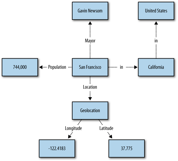
Figure 2-7 shows a graph centered around “San Francisco”. You can see that San Francisco is in California, and California is in the United States. By structuring the places as a graphical hierarchy we avoid the complications of defining a city as being in a state, which is true in some places but not in others. We also have the option to add more information, such as neighborhoods, to the hierarchy if it becomes available. The figure shows various information about San Francisco through relationships to people and numbers and also the city’s geolocation (longitude and latitude), which is important for mapping applications and distance calculations.
You can download a file containing triples about places from http://semprog.com/psw/chapter2/place_triples.txt. In a Python session, load it up and try some simple queries:
>>> from simplegraph import SimpleGraph
>>> placegraph=SimpleGraph()
>>> placegraph.loadfile("place_triples.txt")
This pattern returns everything we know about San Francisco:
>>> for t in placegraph.triples((None,"name","San Francisco")):
...     print t
...
(u'San_Francisco_California', 'name', 'San Francisco')
>>> for t in placegraph.triples(("San_Francisco_California",None,None)):
...     print t
...
('San_Francisco_California', u'name', u'San Francisco')
('San_Francisco_California', u'inside', u'California')
('San_Francisco_California', u'longitude', u'-122.4183')
('San_Francisco_California', u'latitude', u'37.775')
('San_Francisco_California', u'mayor', u'Gavin Newsom')
('San_Francisco_California', u'population', u'744042')
This pattern shows all the mayors in the graph:
>>> for t in placegraph.triples((None,'mayor',None)):
...     print t
...
(u'Aliso_Viejo_California', 'mayor', u'Donald Garcia')
(u'San_Francisco_California', 'mayor', u'Gavin Newsom')
(u'Hillsdale_Michigan', 'mayor', u'Michael Sessions')
(u'San_Francisco_California', 'mayor', u'John Shelley')
(u'Alameda_California', 'mayor', u'Lena Tam')
(u'Stuttgart_Germany', 'mayor', u'Manfred Rommel')
(u'Athens_Greece', 'mayor', u'Dora Bakoyannis')
(u'Portsmouth_New_Hampshire', 'mayor', u'John Blalock')
(u'Cleveland_Ohio', 'mayor', u'Newton D. Baker')
(u'Anaheim_California', 'mayor', u'Curt Pringle')
(u'San_Jose_California', 'mayor', u'Norman Mineta')
(u'Chicago_Illinois', 'mayor', u'Richard M. Daley')

...
We can also try something a little bit more sophisticated by using a loop to get all the cities in California and then getting their mayors:
>>> cal_cities=[p[0] for p in placegraph.triples((None,'inside','California'))]
>>> for city in cal_cities:
...     for t in placegraph.triples((city,'mayor',None)):
...        print t
...
(u'Aliso_Viejo_California', 'mayor', u'William Phillips')
(u'Chula_Vista_California', 'mayor', u'Cheryl Cox')
(u'San_Jose_California', 'mayor', u'Norman Mineta')
(u'Fontana_California', 'mayor', u'Mark Nuaimi')
(u'Half_Moon_Bay_California', 'mayor', u'John Muller')
(u'Banning_California', 'mayor', u'Brenda Salas')
(u'Bakersfield_California', 'mayor', u'Harvey Hall')
(u'Adelanto_California', 'mayor', u'Charley B. Glasper')
(u'Fresno_California', 'mayor', u'Alan Autry')
(etc...)
This is a simple example of joining data in multiple steps. As mentioned previously, the next chapter will show you how to build a simple graph-query language to do all of this in one step.
Celebrities
Our next example is a fun one: celebrities. The wonderful thing about famous people is that other people are always talking about what they’re doing, particularly when what they’re doing is unexpected. For example, take a look at the graph around the ever-controversial Britney Spears, shown in Figure 2-8.
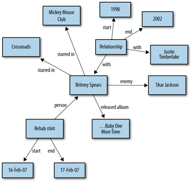
Even from this very small section of Ms. Spears’s life, it’s clear that there are lots of different things and, more importantly, lots of different types of things we say about celebrities. It’s almost comical to think that one could frontload the schema design of everything that a famous musician or actress might do in the future that would be of interest to people. This graph has already failed to include such things as favorite nightclubs, estranged children, angry head-shavings, and cosmetic surgery controversies.
We’ve created a sample file of triples about celebrities at http://semprog.com/psw/chapter2/celeb_triples.txt. Feel free to download this, load it into a graph, and try some fun examples:
>>> from simplegraph import SimpleGraph
>>> cg=SimpleGraph()
>>> cg.load('celeb_triples.csv')
>>> jt_relations=[t[0] for t in cg.triples((None,'with','Justin Timberlake'))]
>>> jt_relations # Justin Timberlake's relationships
[u'rel373', u'rel372', u'rel371', u'rel323', u'rel16', u'rel15',
 u'rel14', u'rel13', u'rel12', u'rel11']
>>> for rel in jt_relations:
...     print [t[2] for t in cg.triples((rel,'with',None))]
...
[u'Justin Timberlake', u'Jessica Biel']
[u'Justin Timberlake', u'Jenna Dewan']
[u'Justin Timberlake', u'Alyssa Milano']
[u'Justin Timberlake', u'Cameron Diaz']
[u'Justin Timberlake', u'Britney Spears']
[u'Justin Timberlake', u'Jessica Biel']
[u'Justin Timberlake', u'Jenna Dewan']
[u'Justin Timberlake', u'Alyssa Milano']
[u'Justin Timberlake', u'Cameron Diaz']
[u'Justin Timberlake', u'Britney Spears']
>>> bs_movies=[t[2] for t in cg.triples(('Britney Spears','starred_in',None))]
>>> bs_movies # Britney Spears' movies
[u'Longshot', u'Crossroads', u"Darrin's Dance Grooves", u'Austin Powers: Goldmember']
>> movie_stars=set()
>>> for t in cg.triples((None,'starred_in',None)):
...     movie_stars.add(t[0])
...
>>> movie_stars # Anyone with a 'starred_in' assertion
set([u'Jenna Dewan', u'Cameron Diaz', u'Helena Bonham Carter', u'Stephan Jenkins',
u'Penxe9lope Cruz', u'Julie Christie', u'Adam Duritz', u'Keira Knightley',
(etc...)
As an exercise, see if you can write Python code to answer some of these questions:
Which celebrities have dated more than one movie star?
Which musicians have spent time in rehab? (Use the
personpredicate from rehab nodes.)Think of a new predicate to represent fans. Add a few assertions about stars of whom you are a fan. Now find out who your favorite stars have dated.
Hopefully you’re starting to get a sense of not only how easy it is to add new assertion types to a triplestore, but also how easy it is to try things with assertions created by someone else. You can start asking questions about a dataset from a single file of triples. The essence of semantic data is ease of extensibility and ease of sharing.
Business
Lest you think that semantic data modeling is all about movies, entertainment, and celebrity rivalries, Figure 2-9 shows an example with a little more gravitas: data from the business world. This graph shows several different types of relationships, such as company locations, revenue, employees, directors, and political contributions.

Obviously, a lot of information that is particular to these businesses could be added to this graph. The relationships shown here are actually quite generic and apply to most companies, and since companies can do so many different things, it’s easy to imagine more specific relationships that could be represented. We might, for example, want to know what investments Berkshire Hathaway has made, or what software products Microsoft has released. This just serves to highlight the importance of a flexible schema when dealing with complex domains such as business.
Again, we’ve provided a file of triples for you to download, at http://semprog.com/psw/chapter2/business_triples.csv. This is a big graph, with 36,000 assertions about 3,000 companies.
Here’s an example session:
>>> from simplegraph import SimpleGraph
>>> bg=SimpleGraph()
>>> bg.load('business_triples.csv')

>>> # Find all the investment banks
>>> ibanks=[t[0] for t in bg.triples((None,'industry','Investment Banking'))]
>>> ibanks
[u'COWN', u'GBL', u'CLMS', u'WDR', u'SCHW', u'LM', u'TWPG', u'PNSN', u'BSC', u'GS',
 u'NITE', u'DHIL', u'JEF', u'BLK', u'TRAD', u'LEH', u'ITG', u'MKTX', u'LAB', u'MS',
 u'MER', u'OXPS', u'SF']

>>> bank_contrib={}  # Contribution nodes from Investment banks
>>> for b in ibanks:
...     bank_contrib[b]=[t[0] for t in bg.triples((None,'contributor',b))]

>>> # Contributions from investment banks to politicians
>>> for b,contribs in bank_contrib.items():
...     for contrib in contribs:
...             print [t[2] for t in bg.triples((contrib,None,None))]

[u'BSC', u'30700.0', u'Orrin Hatch']
[u'BSC', u'168335.0', u'Hillary Rodham Clinton']
[u'BSC', u'5600.0', u'Christopher Shays']
[u'BSC', u'5000.0', u'Barney Frank']
(etc...)

>>> sw=[t[0] for t in bg.triples((None,'industry','Computer software'))]
>>> sw
[u'GOOG', u'ADBE', u'IBM',   # Google, Adobe, IBM

>>> # Count locations
>>> locations={}
>>> for company in sw:
...     for t in bg.triples((company,'headquarters',None)):
...             locations[t[2]]=locations.setdefault(t[2],0)+1

>>> # Locations with 3 or more software companies
>>> [loc for loc,c in locations.items() if c>=3]
[u'Austin_Texas', u'San_Jose_California', u'Cupertino_California',
u'Seattle_Washington']
Notice that we’ve used ticker symbols as IDs, since they are guaranteed to be unique and short.
We hope this gives you a good idea of the many different types of data that can be expressed in triples, the different things you might ask of the data, and how easy it is to extend it. Now let’s move on to creating a better method of querying.