Let’s consider a fragment of the graph represented by the places_triples used in the section Other Examples. We can visualize this graph, representing three cities and the predicates “inside” and “mayor”, as shown in Figure 3-1.

Figure 3-1. A graph of city mayors and locations

Consider the two statements about San Francisco: it is “inside” California, and Gavin Newsom is the mayor. When we express this piece of the graph in triples, we use a common subject identifier San_Francisco_California to indicate that the statements describe a single entity:

("San_Francisco_California", "inside", "California")
("San_Francisco_California", "mayor", "Gavin Newsom")

The shared subject identifier San_Francisco_California indicates that the two statements are about the same entity, the city of San Francisco. When an identifier is used multiple times in a set of triples, it indicates that a node in the graph is shared by all the assertions. And just as you are free to select any name for a variable in a program, the choice of identifiers used in triples is arbitrary, too. As long as you are consistent in your use of an identifier, the facts that you can learn from the assertions will be clear.

For instance, we could have said Gavin Newsom is the mayor of a location within California with the triples:

("foo", "inside", "California")
("foo", "mayor", "Gavin Newsom")

While San_Francisco_California is a useful moniker to help humans understand that “San Francisco” is the location within California that has Newsom as a mayor, the relationships described in the triples using San_Francisco_California and foo are identical.

("foo", "name", "San Francisco")

With an understanding of how shared identifiers are used to indicate shared nodes in the graph, we can return to our question of which mayors serve in California. As before, we start by asking, “Which nodes participate in an assertion with the predicate of ‘inside’ and object of ‘California’?” Using our current query method, we would write this constraint as this triple query:

(None, "inside", "California")

and our query method would return the set of triples that matched the pattern.

Instead of using a wildcard, let’s introduce a variable named ?city to collect the identifiers for the nodes in the graph that satisfy our constraints. For the graph fragment pictured in Figure 3-1 and the triple query pattern ("?city", "inside", "California"), there are two triples that satisfy the constraints, which gives us two possible values for the variable ?city: the identifiers San_Francisco_California and San_Jose_California.

We can express these results as a list of dictionaries mapping the variable name to each matching identifier. We refer to these various possible mappings as “bindings” of the variable ?city to different values. In our example, the results would be expressed as:

[{"?city": "San_Francisco_California"}, {"?city": "San_Jose_California"}]

We now have a way to assign results from a triple query to a variable. We can use this to combine multiple triple queries and take the intersection of the individual result sets. For instance, this query specifies the intersection of two triple queries in order to find all cities in California that have a mayor named Norman Mineta:

("?city", "inside", "California")
("?city", "mayor", "Norman Mineta")

The result [{"?city": "San_Jose_California"}] is the solution to this graph query because it is the only value for the variable ?city that is in all of the individual triple query results. We call the individual triple queries in the graph query “constraints” because each triple query constrains and limits the possible results for the whole graph query.

We can also use variables to ask for more results. By adding an additional variable, we can construct a graph query that tells us which mayors serve cities within California:

("?city", "inside", "California")
("?city", "mayor", "?name_of_mayor")

There are two solutions to this query. In the first solution, the variable ?city is bound to the identifier San_Jose_California, which causes the variable ?name_of_mayor to be bound to the identifier “Norman Mineta”. In the second solution, ?city will be bound to San_Francisco_California, resulting in the variable ?name_of_mayor being bound to “Gavin Newsom”. We can write this solution set as:

[{"?city": "San_Francisco_California", "?name_of_mayor": "Gavin Newsom"}, 
{"?city": "San_Jose_California", "?name_of_mayor": "Norman Mineta"}]

It is important to note that all variables in a solution are bound simultaneously—each dictionary represents an alternative and valid set of bindings given the constraints in the graph query.

In this section, we’ll show you how to add variable binding to your existing triplestore. This will allow you to ask the complex questions in the previous chapter with a single method call, instead of doing separate loops and lookups for each step. For example, the following query returns all of the investment banks in New York that have given money to Utah Senator Orrin Hatch:

>>> bg.query([('?company','headquarters','New_York_NY'),
              ('?company','industry','Investment Banking'),
              ('?company','contributor','?contribution'),
              ('?contribution','recipient','Orrin Hatch'),
              ('?contribution','amount','?dollars')])

The variables are preceded with a question mark, and everything else is considered a constant. This call to the query method tries to find possible values for company, contribution, and dollars that fulfill the following criteria:

From the session at the end of Chapter 2, we know that one possible answer is:

{'?company':'BSC',
 '?contribution':'contXXX',
 '?dollars':'30700'}

If BSC has made multiple contributions to Orrin Hatch, we’ll get a separate solution for each contribution.

Before we get to the implementation, just to make sure you’re clear, here’s another example:

>>> cg.query([('?rel1','with','?person'),
              ('?rel1','with','Britney Spears'),
              ('?rel1','end','?year1'),
              ('?rel2','with','?person'),
              ('?rel2','start','?year1')])

This asks, “Which person started a new relationship in the same year that their relationship with Britney Spears ended?” The question is a little convoluted, but hopefully it shows the power of querying with variable binding. In this case, we’re looking for sets that fulfill the following criteria:

Since there’s nothing saying that person can’t be Britney Spears, it’s possible that she could be one of the answers, if she started a new relationship the same year she ended one. As we look at more sophisticated querying languages, we’ll see ways to impose negative constraints.

The implementation of query is a very simple method for variable binding. It’s not super efficient and doesn’t do any query optimization, but it will work well on the sets we’ve been working with and should help you understand how variable binding works. You can add the following code to your existing simplegraph class, or you can download http://semprog.com/psw/chapter3/simplegraph.py:

    def query(self,clauses):
        bindings = None       
        for clause in clauses:
            bpos = {}
            qc = []
            for pos, x in enumerate(clause):
                if x.startswith('?'):
                    qc.append(None)
                    bpos[x] = pos
                else:
                    qc.append(x)
            rows = list(self.triples((qc[0], qc[1], qc[2])))
            if bindings == None:
                # This is the first pass, everything matches
                bindings = []
                for row in rows:   
                    binding = {}
                    for var, pos in bpos.items():
                        binding[var] = row[pos]
                    bindings.append(binding)
            else:
                # In subsequent passes, eliminate bindings that don't work
                newb = []
                for binding in bindings:
                    for row in rows:
                        validmatch = True
                        tempbinding = binding.copy()
                        for var, pos in bpos.items():
                            if var in tempbinding:
                                if tempbinding[var] != row[pos]:
                                    validmatch = False
                            else:
                                tempbinding[var] = row[pos]
                        if validmatch: newb.append(tempbinding)
                bindings = newb    
        return bindings

This method loops over each clause, keeping track of the positions of the variables (any string that starts with ?). It replaces all the variables with None so that it can use the triples method already defined in simplegraph. It then gets all the rows matching the pattern with the variables removed.

For every row in the set, it looks at the positions of the variables in the clause and tries to fit the values to one of the existing bindings. The first time through there are no existing bindings, so every row that comes back becomes a potential binding. After the first time, each row is compared to the existing bindings—if it matches, more variables are added and the binding is added to the current set. If there are no rows that match an existing binding, that binding is removed.

Try using this new query method in a Python session for the two aforementioned queries:

>>> from simplegraph import SimpleGraph()
>>> bg = SimpleGraph()
>>> bg.load('business_triples.csv')
>>> bg.query([('?company','headquarters','New_York_New_York'),
              ('?company','industry','Investment Banking'),
              ('?cont','contributor','?company'),
              ('?cont','recipient','Orrin Hatch'),
              ('?cont','amount','?dollars')])
[{'company': u'BSC', 'cont': u'contrib285', 'dollars': u'30700.0'}]
>>> cg = SimpleGraph()
>>> cg.load('celeb_triples.csv')
>>> cg.query([('?rel1','with','?person'),
              ('?rel1','with','Britney Spears'),
              ('?rel1','end','?year1'),
              ('?rel2','with','?person'),
              ('?rel2','start','?year1')])
[{'person': u'Justin Timberlake', 'rel1': u'rel16', 'year1': u'2002', 
    'rel2': u'rel372'} ...

Now see if you can formulate some queries of your own on the movie graph. For example, which actors have starred in movies directed by Ridley Scott as well as movies directed by George Lucas?

The basic pattern of inference is simply to query for information (in the form of bindings) relevant to a rule, then apply a transformation that turns these bindings into a new set of triples that get added back to the triplestore. We’re going to create a basic class that defines inference rules, but first we’ll add a new method for applying rules to the SimpleGraph class. If you downloaded http://semprog.com/psw/chapter3/simplegraph.py, you should already have this method. If not, add it to your class:

    def applyinference(self,rule):
        queries = rule.getqueries()
        bindings=[]
        for query in queries:
            bindings += self.query(query)
        for b in bindings:
            new_triples = rule.maketriples(b)
            for triple in new_triples:
                self.add(triple)

This method takes a rule (usually an instance of InferenceRule) and runs its query to get a set of bindings. It then calls rule.maketriples on each set of bindings, and adds the returned triples to the store.

The InferenceRule class itself doesn’t do much, but it serves as a base from which other rules can inherit. Child classes will override the getquery method and define a new method called _maketriples, which will take each binding as a parameter. You can download http://semprog.com/psw/chapter3/inferencerule.py, which contains the class definition of InferenceRule and the rest of the code from this section. If you prefer, you can create a new file called inferencerule.py and add the following code:

class InferenceRule:
    def getqueries(self):
        return []
    
    def maketriples(self,binding):
        return self._maketriples(**binding)

Now we are ready to define a new rule. Our first rule will identify companies headquartered in cities on the west coast of the United States and identify them as such:

class WestCoastRule(InferenceRule):
    def getqueries(self):
        sfoquery = [('?company', 'headquarters', 'San_Francisco_California')]
        seaquery = [('?company', 'headquarters', 'Seattle_Washington')]
        laxquery = [('?company', 'headquarters', 'Los_Angelese_California')]
        porquery = [('?company', 'headquarters', 'Portland_Oregon')]
        return [sfoquery, seaquery, laxquery, porquery]

    def _maketriples(self, company):
        return [(company, 'on_coast', 'west_coast')]

The rule class lets you define several queries: in this case, there’s a separate query for each of the major west coast cities. The variables used in the queries themselves (in this case, just company) become the parameters for the call to _maketriples. This rule asserts that all the companies found by the first set of queries are on the west coast.

You can try this in a session:

>>> wcr = WestCoastRule()
>>> bg.applyinference(wcr)
>>> list(bg.triples((None, 'on_coast', None)))
[(u'PCL', 'on_coast', 'west_coast'), (u'PCP', 'on_coast', 'west_coast') ...

Although we have four different queries for our west coast rule, each of them has only one clause, which makes the rules themselves very simple. Here’s a rule with a more sophisticated query that can be applied to the celebrities graph:

class EnemyRule(InferenceRule):
    def getqueries(self):
        partner_enemy = [('?person', 'enemy', '?enemy'),
                         ('?rel', 'with', '?person'),
                         ('?rel', 'with', '?partner)]
        return [partner_enemy]

    def _maketriples(self, person, enemy, rel, partner):
        return (partner, 'enemy', enemy)

Just from looking at the code, can you figure out what this rule does? It asserts that if a person has a relationship partner and also an enemy, then their partner has the same enemy. That may be a little presumptuous, but nonetheless it demonstrates a simple logical rule that you can make with this pattern. Again, try it in a session:

>>> from simplegraphq import *
>>> cg = SimpleGraph()
>>> cg.load('celeb_triples.csv')
>>> er = EnemyRule()
>>> list(cg.triples((None, 'enemy', None)))
[(u'Jennifer Aniston', 'enemy', u'Angelina Jolie')...
>>> cg.applyinference(er)
>>> list(cg.triples((None, 'enemy', None)))
[(u'Jennifer Aniston', 'enemy', u'Angelina Jolie'), (u'Vince Vaughn', 'enemy', 
    u'Angelina Jolie')...

These queries are all a little self-directed, since they operate directly on the data and have limited utility. We’ll now see how we can use this reasoning framework to add more information to the triplestore by retrieving it from outside sources.

Geocoding is the process of taking an address and getting the geocoordinates (the longitude and latitude) of that address. When you use a service that shows the location of an address on a map, the address is always geocoded first. Besides displaying on a map, geocoding is useful for figuring out the distance between two places and determining automatically if an address is inside or outside particular boundaries. In this section, we’ll show you how to use an external geocoder to infer triples from addresses of businesses.

38.898748,-77.037684,1600 Pennsylvania Ave NW,Washington,DC,20502

from urllib import urlopen, quote_plus

class GeocodeRule(InferenceRule):
    def getquery(self):
        return [('?place', 'address', '?address')]
    
    def _maketriples(self, place, address):
        url = 'http://rpc.geocoder.us/service/csv?address=%s' % quote_plus(address)
        con = urlopen(url)
        data = con.read()
        con.close()        
        parts = data.split(',')
        if len(parts) >= 5:
            return [(place, 'longitude', parts[0]),
                    (place, 'latitude', parts[1])]
        else:
            # Couldn't geocode this address
            return []

>>> from simplegraph import *
>>> from inferencerule import *
>>> geograph = SimpleGraph()
>>> georule = GeocodeRule()
>>> geograph.add(('White House', 'address', '1600 Pennsylvania Ave, Washington, DC'))
>>> list(geograph.triples((None, None, None))
[('White House', 'address', '1600 Pennsylvania Ave, Washington, DC')]
>>> geograph.applyinference(georule)
>>> list(geograph.triples((None, None, None))
[('White House', 'latitude', '-77.037684'),
 ('White House', 'longitude', '38.898748'),
 ('White House', 'address', '1600 Pennsylvania Ave, Washington, DC')]

The fact that these inferences create new assertions in the triplestore is incredibly useful to us. It means that we can write inference rules that operate on the results of other rules without explicitly coordinating all of the rules together. This allows the creation of completely decoupled, modular systems that are very robust to change and failure.

To understand how this works, take a look at CloseToRule. This takes a place name and a graph in its constructor. It queries for every geocoded item in the graph, calculates how far away they are, and then asserts close_to for all of those places that are close by:

class CloseToRule(InferenceRule):
    
    def __init__(self, place, graph):
        self.place = place
        laq = list(graph.triples((place, 'latitude', None)))
        loq = list(graph.triples((place, 'longitude', None)))
        
        if len(laq) == 0 or len(loq) == 0:
            raise "Exception","%s is not geocoded in the graph" % place
        
        self.lat = float(laq[0][2])
        self.long = float(loq[0][2])
    
    def getqueries(self):
        geoq=[('?place', 'latitude', '?lat'), ('?place', 'longitude', '?long')]
        return [geoq]
    
    def _maketriples(self, place, lat, long):
        # Formula for distance in miles from geocoordinates
        distance=((69.1*(self.lat - float(lat)))**2 + 
            (53*(self.lat - float(lat)))**2)**.5
        
        # Are they less than a mile apart
        if distance < 1:
            return [(self.place, 'close_to', place)]
        else:
            return [(self.place, 'far_from', place)]

Now you can use these two rules together to first geocode the addresses, then create assertions about which places are close to the White House:

>>> from simplegraph import *
>>> from inferencerule import *
>>> pg = SimpleGraph()
>>> pg.load('DC_addresses.csv')
>>> georule = GeocodeRule()
>>> pg.applyinference(georule)
>>> whrule = CloseToRule('White House',pg)
>>> pg.applyinference(whrule)
>>> list(pg.triples((None, 'close_to', None)))
[('White House', 'close_to', u'White House'), 
 ('White House', 'close_to', u'Pot Belly'),
 ('White House', 'close_to', u'Equinox')]

Now we’ve chained together two rules. Keep this session open while we take a look at another rule, which identifies restaurants that are likely to be touristy. In the DC_addresses file, there are assertions about what kind of place each venue is (“tourist attraction” or “restaurant”) and also information about prices (“cheap” or “expensive”). The TouristyRule combines all this information along with the close_to assertions to determine which restaurants are touristy:

class TouristyRule(InferenceRule):
    def getqueries(self):
        tr = [('?ta', 'is_a', 'Tourist Attraction'),
              ('?ta', 'close_to', '?restaurant'),
              ('?restaurant', 'is_a', 'restaurant'),
              ('?restaurant', 'cost', 'cheap')]
            
    def _maketriples(self, ta, restaurant):
        return [(restaurant, 'is_a', 'touristy restaurant')]

That is, if a restaurant is cheap and close to a tourist attraction, then it’s probably a pretty touristy restaurant:

>>> tr = TouristyRule()
>>> pg.applyinference(tr)
>>> list(pg.triples((None, 'is_a', 'touristy restaurant')))
[(u'Pot Belly', 'is_a', 'touristy restaurant')]

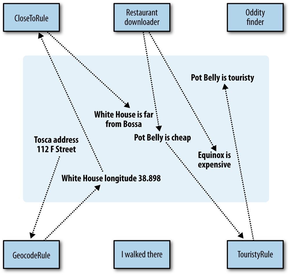
So we’ve gone from a bunch of addresses and restaurant prices to predictions about restaurants where you might find a lot of tourists. You can think of this as a group of dependent functions, similar to Figure 3-2, which represents the way we normally think about data processing.

Figure 3-2. A “chain view” of the rules

What’s important to realize here is that the rules exist totally independently. Although we ran the three rules in sequence, they weren’t aware of each other—they just looked to see if there were any triples that they knew how to deal with and then created new ones based on those. These rules can be run continuously—even from different machines that have access to the same triplestore—and still work properly, and new rules can be added at any time. To help understand what this implies, consider a few examples:

So a better way to think about this is Figure 3-3.

The rules all share an information store and look for information they can use to generate new information. This is sometimes referred to as a multi-agent blackboard. It’s a different way of thinking about programming that sacrifices in efficiency but that has the advantages of being very decoupled, easily distributable, fault tolerant, and flexible.

Figure 3-3. Inference rules reading from and writing to a “blackboard”

It’s important to realize, of course, that “intelligence” doesn’t come from chains of symbolic logic like this. In the past, many people have made the mistake of trying to generate intelligent behavior this way, attempting to model large portions of human knowledge and reasoning processes using only symbolic logic. These approaches always reveal that there are pretty severe limitations on what can be modeled. Predicates are imprecise, so many inferences are impossible or are only correct in the context of a particular application.

The examples here show triggers for making new assertions entirely from existing ones, and also show ways to query other sources to create new assertions based on existing ones.

A good example of the breadth-first search algorithm is the trivia game “Six Degrees of Kevin Bacon,” where one player names a film actor, and the other player tries to connect that actor to the actor Kevin Bacon through the shortest path of movies and co-stars. For instance, one answer for the actor Val Kilmer would be that Val Kilmer starred in Top Gun with Tom Cruise, and Tom Cruise starred in A Few Good Men with Kevin Bacon, giving a path of length 2 because two movies had to be traversed. See Figure 3-4.

Figure 3-4. Breadth-first search from Val Kilmer to Kevin Bacon

Here’s an implementation of breadth-first search over the movie data introduced in Chapter 2. On each iteration of the while loop, the algorithm processes a successive group of nodes one edge further than the last. So on the first iteration, the starting actor node is examined, and all of its adjacent movies that have not yet been seen are added to the movieIds list. Then all of the actors in those movies are found and are added to the actorIds list if they haven’t yet been seen. If one of the actors is the one we are looking for, the algorithm finishes.

The shortest path back to the starting node from each examined node is stored at each step as well. This is done in the “parent” variable, which at each step points to the node that was used to find the current node. This path of “parent” nodes can be followed back to the starting node:

def moviebfs(startId, endId, graph):
    actorIds = [(startId, None)]
    # keep track of actors and movies that we've seen:
    foundIds = set()
    iterations = 0
    while len(actorIds) > 0:
        iterations += 1
        print "Iteration " + str(iterations)
        # get all adjacent movies:
        movieIds = []
        for actorId, parent in actorIds:
            for movieId, _, _ in graph.triples((None, "starring", actorId)): 
                if movieId not in foundIds: 
                    foundIds.add(movieId)
                    movieIds.append((movieId, (actorId, parent)))
        # get all adjacent actors:
        nextActorIds = []
        for movieId, parent in movieIds:
            for _, _, actorId in graph.triples((movieId, "starring", None)): 
                if actorId not in foundIds: 
                    foundIds.add(actorId)
                    # we found what we're looking for:
                    if actorId == endId: return (iterations, (actorId, 
                        (movieId, parent)))
                    else: nextActorIds.append((actorId, (movieId, parent)))
        actorIds = nextActorIds
    # we've run out of actors to follow, so there is no path:
    return (None, None)

Now we can define a function that runs moviebfs and recovers the shortest path:

def findpath(start, end, graph):
    # find the ids for the actors and compute bfs:
    startId = graph.value(None, "name", start)
    endId = graph.value(None, "name", end)
    distance, path = moviebfs(startId, endId, graph)
    print "Distance: " + str(distance)
    # walk the parent path back to the starting node:
    names = []
    while path is not None:
        id, nextpath = path
        names.append(graph.value(id, "name", None))
        path = nextpath
    print "Path: " + ", ".join(names)

Here’s the output for Val Kilmer, Bruce Lee, and Harrison Ford. (Note that our movie data isn’t as complete as some databases on the Internet, so there may in fact be a shorter path for some of these actors.)

>>> import simplegraph
>>> graph = simplegraph.SimpleGraph()
>>> graph.load("movies.csv")
>>> findpath("Val Kilmer", "Kevin Bacon", graph)
Iteration 1
Iteration 2
Distance: 2
Path: Kevin Bacon, A Few Good Men, Tom Cruise, Top Gun, Val Kilmer
>>> findpath("Bruce Lee", "Kevin Bacon", graph)
Iteration 1
Iteration 2
Iteration 3
Distance: 3
Path: Kevin Bacon, The Woodsman, David Alan Grier, A Soldier's Story, Adolph Caesar, 
    Fist of Fear, Touch of Death, Bruce Lee
>>> findpath("Harrison Ford", "Kevin Bacon", graph)
Iteration 1
Iteration 2
Distance: 2
Path: Kevin Bacon, Apollo 13, Kathleen Quinlan, American Graffiti, Harrison Ford

The triples provided for the business and places graphs both contain city names referring to places in the United States. To make the join easy, we already normalized the city names so that they’re all written as City_State, e.g., San_Francisco_California or Omaha_Nebraska. In a session, you can look at assertions that are in the two separate graphs:

>>> from simplegraph import SimpleGraph
>>> bg=SimpleGraph()
>>> bg.load('business_triples.csv')
>>> pg=SimpleGraph()
>>> pg.load('place_triples.csv')

>>> for t in bg.triples((None, 'headquarters', 'San_Francisco_California')):
...     print t
(u'URS', 'headquarters', 'San_Francisco_California')
(u'PCG', 'headquarters', 'San_Francisco_California')
(u'CRM', 'headquarters', 'San_Francisco_California')
(u'CNET', 'headquarters', 'San_Francisco_California')
(etc...)

>>> for t in pg.triples(('San_Francisco_California', None, None)):
...     print t
('San_Francisco_California', u'name', u'San Francisco')
('San_Francisco_California', u'inside', u'California')
('San_Francisco_California', u'longitude', u'-122.4183')
('San_Francisco_California', u'latitude', u'37.775')
('San_Francisco_California', u'mayor', u'Gavin Newsom')
('San_Francisco_California', u'population', u'744042')

We’re going to merge the data from the places graph, such as population and location, into the business graph. This is pretty straightforward—all we need to do is generate a list of places where companies are headquartered, find the equivalent nodes in the places graph, and copy over all their triples. Try this in your Python session:

>>> hq=set([t[2] for t in bg.triples((None,'headquarters',None))])
>>> len(hq)
889
>>> for pt in pg.triples((None, None, None)):
...     if pt[0] in hq: bg.add(pt)

Congratulations—you’ve successfully integrated two distinct datasets! And you didn’t even have to worry about their schemas.

This may not seem like much yet, but you can now construct queries across both graphs, using the constraint-based querying code from this chapter. For example, you can now get a summary of places where software companies are headquartered:

>>> results = bg.query([('?company', 'headquarters', '?city'),
                        ('?city', 'inside', '?region'),
                        ('?company', 'industry', 'Computer software')])
>>> [r['region'] for r in results]
[u'San_Francisco_Bay_Area', u'California', u'United_States', u'Silicon_Valley', 
    u'Northern_California' ...

You can also search for investment banks that are located in cities with more than 1,000,000 people:

>>> results = bg.query([('?company', 'headquarters', '?city'),
                        ('?city', 'population', '?pop'),
                        ('?company', 'industry', 'Investment banking')])
>>> [r for r in results if int(r['pop']) > 1000000]
[{'city': u'Chicago_Illinois', 'company': u'CME', 'pop': u'2833321'}, ...

This is just a small taste of what’s possible. Later we’ll see how the “semantic web” envisions merging thousands of graphs, which will allow for extremely sophisticated queries across data from many sources.

Graphviz is a free software package created by AT&T. It takes simple files describing nodes and connections and applies layout and edge-routing algorithms to produce an image in one of several possible formats. You can download Graphviz from http://www.graphviz.org/.

The input files are in a format called DOT, which is a simple text format that looks like this:

graph "test" {
    A -- B;
    A -- C;
    C -- D;
}

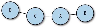
This graph has four nodes: A, B, C, and D. A is connected to B and C, and C is connected to D. There are two different layout programs that come with Graphviz, called dot and neato. Dot produces hierarchical layouts for trees, and neato (which we’ll be using in this section) produces layouts for nonhierarchical graphs. The output from neato for the previous example is shown in Figure 3-5.

Figure 3-5. Visualization of the ABCD graph

There are a lot of different settings for DOT files, to adjust things like node size, edge thickness, colors, and layout options. We won’t cover them all here, but you can find a complete description of the file format in the documentation at http://www.graphviz.org/pdf/dotguide.pdf.

The first thing we want to try is creating a graph of a subset of triples. You can download the code for this section at http://semprog.com/psw/chapter3/graphtools.py; alternatively, you can create a file called graphtools.py and add the triplestodot function:

def triplestodot(triples, filename):
    out=file(filename, 'w')
    out.write('graph "SimpleGraph" {
')
    
    out.write('overlap = "scale";
')
    for t in triples:
         out.write('"%s" -- "%s" [label="%s"]
' % (t[0].encode('utf-8'),
                                                    t[2].encode('utf-8'),
                                                    t[1].encode('utf-8')))
    out.write('}')

This function simply takes a set of triples, which you would retrieve using the triples method of any graph. It creates a DOT file containing those same triples, to be used by Graphviz. Let’s try it on the celebrity graph using triples about relationships. In your Python session:

>>> from simplegraph import *
>>> from graphtools import *
>>> cg = SimpleGraph()
>>> cg.load('celeb_triples.csv')
>>> rel_triples = cg.triples((None, 'with', None))
>>> triplestodot(rel_triples, 'dating_triples.dot')

This should save a file called dating_triples.dot. To convert it to an image, you need to run neato from the command line:

$ neato -Teps -Odating_triples dating_triples.dot

This will save an Encapsulated PostScript (EPS) file called dating_triples.eps, which will look something like what you see in Figure 3-6.

Figure 3-6. Visualization of raw triples in the celebrity dating set

Try generating other images, perhaps a completely unfiltered version that contains every assertion in the graph. You can also try generating images of the other sample data that we’ve provided.

The problem with graphing the dating triples is that although the graph shows the exact structure of the data, the “rel” nodes shown don’t offer any additional information and simply clutter the graph. If we’re willing to assume that a relationship is always between two people, then we can eliminate those nodes entirely and connect the people directly to one another. This is pretty easy to do using the query language that we devised at the start of this chapter. The file graphtools.py also contains a method called querytodot, which takes a query and two variable names:

def querytodot(graph, query, b1, b2, filename):
    out=file(filename, 'w')
    out.write('graph "SimpleGraph" {
')
    out.write('overlap = "scale";
')
    results = graph.query(query)
    donelinks = set()
    for binding in results:
        if binding[b1] != binding[b2]:
            n1, n2 = binding[b1].encode('utf-8'), binding[b2].encode('utf-8')
            if (n1, n2) not in donelinks and (n2, n1) not in donelinks:
                out.write('"%s" -- "%s"
' % (n1, n2))
                donelinks.add((n1, n2))
    out.write('}')

This method queries the graph using the provided query, then loops over the resulting bindings, pulling out the variables b1 and b2 and creating a link between them. We can use this method to create a much cleaner celebrity dating graph:

>>> from simplegraph import *
>>> from graphtools import *
>>> cg = SimpleGraph()
>>> cg.load('celeb_triples.csv')
>>> querytodot(cg, [('?rel', 'with', '?p1'), ('?rel', 'with', '?p2')], 'p1', 
    'p2', 'relationships.dot')
>>> exit()
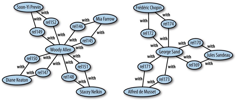
$ neato -Teps -Orelationships relationships.dot

A partial result is shown in Figure 3-7.

Figure 3-7. Viewing the celebrity dating graph

See if you can make other images from the business or movie data. For example, try graphing all the contributors to different politicians.